1. No category

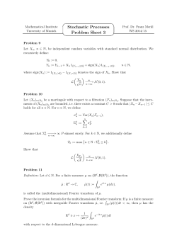
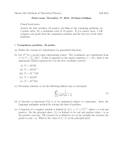
285
4.6 Applications of Transforms to Differential Equations
19. Establish the following result by formally inverting the Laplace transform
1 sinh(sy)
ˆ
F(s)
=
s sinh(sℓ)
ℓ>0
∞
y ! 2(−1)n
f (x) = +
sin
ℓ n=1 nπ
"
nπ y
ℓ
#
cos
"
nπ x
ℓ
#
See the remark at the end of Problem 18, which explains how to show
how the inverse Laplace transform can be proven to be valid in a situation
such as this where there are an infinite number of poles.
∗
4.6 Applications of Transforms to Differential Equations
A particularly valuable technique available to solve differential equations in
infinite and semiinfinite domains is the use of Fourier and Laplace transforms.
In this section we describe some typical examples. The discussion is not intended to be complete. The aim of this section is to elucidate the transform
technique, not to detail theoretical aspects regarding differential equations. The
reader only needs basic training in the calculus of several variables to be able
to follow the analysis. We shall use various classical partial differential equations (PDEs) as vehicles to illustrate methodology. Herein we will consider
well-posed problems that will yield unique solutions. More general PDEs and
the notion of well-posedness are investigated in considerable detail in courses
on PDEs.
Example 4.6.1 Steady state heat flow in a semiinfinite domain obeys Laplace’s
equation. Solve for the bounded solution of Laplace’s equation
∂ 2 φ(x, y) ∂ 2 φ(x, y)
+
=0
∂x2
∂ y2
(4.6.1)
in the region −∞ < x < ∞, y$ > 0, where on y = 0 we
$ ∞are given2 φ(x, 0) =
∞
1
2
h(x) with h(x) ∈ L ∩ L (i.e., −∞ |h(x)| d x < ∞ and −∞ |h(x)| d x < ∞).
This example will allow us to solve Laplace’s Equation (4.6.1) by Fourier
ˆ
transforms. Denoting the Fourier transform in x of φ(x, y) as Φ(k,
y):
ˆ
Φ(k,
y) =
%
∞
e−ikx φ(x, y) d x
−∞
taking the Fourier transform of Eq. (4.6.1), and using the result from Section 4.5
for the Fourier transform of derivatives, Eqs. (4.5.16a,b) (assuming the validity
286
4 Residue Calculus and Applications of Contour Integration
of interchanging y-derivatives and integrating over k, which can be verified
a posteriori), we have
ˆ
∂ 2Φ
ˆ =0
− k2Φ
∂ y2
(4.6.2)
Hence
ˆ
Φ(k,
y) = A(k)eky + B(k)e−ky
where A(k) and B(k) are arbitrary functions of k, to be specified by the boundary
ˆ
conditions. We require that Φ(k,
y) be bounded for all y > 0. In order that
ˆ
Φ(k,
y) yield a bounded function φ(x, y), we need
ˆ
Φ(k,
y) = C(k)e−|k|y
(4.6.3)
ˆ (k) fixes C(k) = H
ˆ (k),
Denoting the Fourier transform of φ(x, 0) = h(x) by H
so that
ˆ
ˆ (k)e−|k|y
Φ(k,
y) = H
(4.6.4)
From Eq. (4.5.1) by direct integration (contour integration is not necessary) we
y
ˆ
find that F(k,
y) = e−|k|y is the Fourier transform of f (x, y) = π1 x 2 +y
2 , thus
from the convolution formula Eq. (4.5.17) the solution to Eq. (4.6.1) is given by
1
φ(x, y) =
π
!
∞
−∞
y h(x ′ )
dx′
′
2
2
(x − x ) + y
(4.6.5)
If h(x) were taken to be a Dirac delta function concentrated at x = ζ , h(x) =
ˆ (k) = e−ikζ , and from Eq. (4.6.4) directly (or
h s (x − ζ ) = δ(x − ζ ), then H
Eq. (4.6.5)) a special solution to Eq. (4.6.1), φs (x, y) is
1
φs (x, y) = G(x − ζ, y) =
π
"
y
(x − ζ )2 + y 2
#
(4.6.6)
Function G(x − ζ, y) is called a Green’s function; it is a fundamental solution
to Laplace’s equation in this region. Green’s functions have the property of
solving a given equation with delta function inhomogeneity. From the boundary
values h s (x − ζ, 0) = δ(x − ζ ) we may construct arbitrary initial values
φ(x, 0) =
!
∞
−∞
h(ζ ) δ(x − ζ ) dζ = h(x)
(4.6.7a)
4.6 Applications of Transforms to Differential Equations
287
and, because Laplace’s equation is linear, we find by superposition that the
general solution satisfies
φ(x, y) =
!
∞
−∞
h(ζ ) G(x − ζ, y) dζ
(4.6.7b)
which is Eq. (4.6.5), noting that ζ or x ′ are dummy integration variables. In
many applications it is sufficient to obtain the Green’s function of the underlying
differential equation.
The formula (4.6.5) is sometimes referred to as the Poisson formula for a
half plane. Although we derived it via transform methods, it is worth noting
that a pair of such formulae can be derived from Cauchy’s integral formula. We
describe this alternative method now. Let f (z) be analytic on the real axis and
in the upper half plane and assume f (ζ ) → 0 uniformly as ζ → ∞. Using a
large closed semicircular contour such as that depicted in Figure 4.2.1 we have
1
f (z) =
2πi
1
0=
2πi
"
C
"
C
f (ζ )
dζ
ζ −z
f (ζ )
dζ
ζ − z¯
where Im z > 0 (in the second formula there is no singularity because the
contour closes in the upper half plane and ζ = z¯ in the lower half plane).
Adding and subtracting yields
1
f (z) =
2πi
"
C
#
$
1
1
f (ζ )
±
dζ
ζ −z
ζ − z¯
The semicircular portion of the contour C R vanishes as R → ∞, implying
the following on Im ζ = 0 for the plus and minus parts of the above integral,
respectively: calling z = x + i y and ζ = x ′ + i y ′ ,
$
x′ − x
f (x , y = 0)
dx′
′
2
2
(x − x ) + y
−∞
#
$
!
1 ∞
y
′
′
dx′
f (x, y) =
f (x , y = 0)
π −∞
(x − x ′ )2 + y 2
1
f (x, y) =
πi
!
∞
′
′
#
Calling
f (z) = f (x, y) = u(x, y) + i v(x, y),
Re f (x, y = 0) = u(x, 0) = h(x)
288
4 Residue Calculus and Applications of Contour Integration
and taking the imaginary part of the first and the real part of the second of the
above formulae, yields the conjugate Poisson formulae for a half plane:
−1
v(x, y) =
π
1
u(x, y) =
π
!
∞
−∞
!
∞
−∞
"
h(x )
′
"
h(x )
′
x′ − x
(x − x ′ )2 + y 2
y
(x − x ′ )2 + y 2
#
#
dx′
dx′
Identifying u(x, y) as φ(x, y), we see that the harmonic function u(x, y) (because f (z) is analytic its real and imaginary parts satisfy Laplace’s equation) is
given by the same formula as Eq. (4.6.5). Moreover, we note that the imaginary
part of f (z), v(x, y), is determined by the real part of f (z) on the boundary.
We see that we cannot arbitrarily prescribe both the real and imaginary parts
of f (z) on the boundary. These formulae are valid for a half plane. Similar
formulae can be obtained by this method for a circle (see also Example 10,
Section 2.6).
Laplace’s equation, (4.6.1), is typical of a steady state situation, for example,
as mentioned earlier, steady state heat flow in a uniform metal plate. If we have
time-dependent heat flow, the diffusion equation
∂φ
= k∇ 2 φ
∂t
(4.6.8)
is a relevant equation with k the diffusion coefficient. In Eq. (4.6.8), ∇ 2 is the
2
2
Laplacian operator, which in two dimensions is given by ∇ 2 = ∂∂x 2 + ∂∂y 2 . In
one dimension, taking k = 1 for convenience, we have the following initial
value problem:
∂φ(x, t)
∂ 2 φ(x, t)
=
∂t
∂x2
(4.6.9)
The Green’s function for the problem on the line −∞ < x < ∞ is obtained
by solving Eq. (4.6.9) subject to
φ(x, 0) = δ(x − ζ )
Example 4.6.2 Solve for the Green’s function of Eq. (4.6.9). Define
ˆ
Φ(k,
t) =
!
∞
−∞
e−ikx φ(x, t) d x
4.6 Applications of Transforms to Differential Equations
289
whereupon the Fourier transform of Eq. (4.6.9) satisfies
ˆ
∂ Φ(k,
t)
ˆ
= −k 2 Φ(k,
t)
∂t
(4.6.10)
2
2
ˆ
ˆ
Φ(k,
t) = Φ(k,
0)e−k t = e−ikζ −k t
(4.6.11)
hence
ˆ
where Φ(k,
0) = e−ikζ is the Fourier transform of φ(x, 0) = δ(x − ζ ). Thus,
by the inverse Fourier transform, and calling G(x − ζ, t) the inverse transform
of (4.6.11),
1
G(x − ζ, t) =
2π
=e
!
∞
2
eik(x−ζ )−k t dk
−∞
−(x−ζ )2 /4t
1
·
2π
!
∞
e−(k−i
x−ζ 2
2t ) t
dk
−∞
(x−ζ )2
e− 4t
= √
(4.6.12)
2 πt
"∞
√
2
where we use −∞ e−u du = π. Arbitrary initial values are included by
again observing that
φ(x, 0) = h(x) =
!
∞
−∞
h(ζ )δ(x − ζ ) dζ
which implies
!
∞
1
φ(x, t) =
G(x − ζ, t)h(ζ ) dζ = √
2 πt
−∞
!
∞
h(ζ ) e−
(x−ζ )2
4t
dζ (4.6.13)
−∞
The above solution to Eq. (4.6.9) could also be obtained by using Laplace
transforms. It is instructive to show how the method proceeds in this case. We
begin by introducing the Laplace transform of φ(x, t) with respect to t:
ˆ
Φ(x,
s) =
!
∞
e−st φ(x, t) dt
(4.6.14)
0
Taking the Laplace transform in t of Eq. (4.6.8), with φ(x, 0) = δ(x − ζ ),
yields
ˆ
∂ 2Φ
ˆ
(x, s) − s Φ(x,
s) = −δ(x − ζ )
∂x2
(4.6.15)
290
4 Residue Calculus and Applications of Contour Integration
Hence the Laplace transform of the Green’s function to Eq. (4.6.9) satisfies
Eq. (4.6.15). We remark that generally speaking, any function G(x − ζ ) satisfying
LG(x − ζ ) = −δ(x − ζ )
where L is a linear differential operator, is referred to as a Green’s function. The
general solution
! ∞ corresponding to φ(x, 0) = h(x) is obtained by superposition:
φ(x, t) = −∞ G(x − ζ )h(ζ ) dζ . Equation (4.6.15) is solved by first finding
the bounded homogeneous solutions on −∞ < x < ∞, for (x − ζ ) > 0 and
(x − ζ ) < 0:
ˆ + (x − ζ, s) = A(s)e−s 1/2 (x−ζ )
Φ
ˆ − (x − ζ, s) = B(s)es
Φ
1/2
for x − ζ > 0
for x − ζ < 0
(x−ζ )
(4.6.16)
where we take s 1/2 to have a branch cut on the negative real axis; that is,
s = r eiθ , −π ≤ θ < π . This will allow us to readily invert the Laplace transform (Re s > 0).
The coefficients A(s) and B(s) in Eq. (4.6.16) are found by (a) requiring
ˆ − ζ, s) at x = ζ and by (b) integrating Eq. (4.6.15) from
continuity of Φ(x
x = ζ − ϵ, to x = ζ + ϵ, and taking the limit as ϵ → 0+ . This yields a jump
ˆ
condition on ∂∂(x (x − ζ, s):
" ˆ
#x−ζ =0+
∂Φ
(x − ζ, s)
= −1
∂x
x−ζ =0−
(4.6.17)
Continuity yields A(s) = B(s), and Eq. (4.6.17) gives
−s 1/2 A(s) − s 1/2 B(s) = −1
(4.6.18a)
hence
A(s) = B(s) =
1
2s 1/2
(4.6.18b)
ˆ − ζ, s) is written in the compact form:
Using Eq. (4.6.16), Φ(x
1/2
−s |x−ζ |
ˆ − ζ, s) = e
Φ(x
2s 1/2
(4.6.19)
The solution φ(x, t) is found from the inverse Laplace transform:
1
φ(x, t) =
2πi
$
c+i∞
c−i∞
e−s
1/2
|x−ζ | st
2s 1/2
e
ds
(4.6.20)
4.6 Applications of Transforms to Differential Equations
291
for c > 0. To evaluate Eq. (4.6.20), we employ the same keyhole contour as
in Example 4.5.3 in Section 4.5 (see Figure 4.5.2). There are no singularities
enclosed, and the contours C R and Cϵ at infinity and at the origin vanish in the
limit R → ∞, ϵ → 0, respectively. We only obtain contributions along the
top and bottom of the branch cut to find
−1
φ(x, t) =
2πi
!
1/2
0
e−ir |x−ζ | e−r t iπ
e dr
2r 1/2 eiπ/2
∞
!
−1
+
2πi
∞
0
1/2
eir |x−ζ | e−r t −iπ
e
dr
2r 1/2 e−iπ/2
(4.6.21)
In the second integral we put r 1/2 = u; in the first we put r 1/2 = u and then take
u → −u, whereupon we find the same answer as before (see Eq. (4.6.12)):
1
φ(x, t) =
2π
!
1
=
2π
!
∞
e−u
2
t+iu|x−ζ |
du
−∞
∞
e−(u−i
|x−ζ | 2
2t ) t
e−
(x−ζ )2
4t
du
−∞
2
e−(x−ζ ) /4t
√
=
2 πt
(4.6.22)
The Laplace transform method can also be applied to problems in which the
spatial variable is on the semiinfinite domain. However, rather than use Laplace
transforms, for variety and illustration, we show below how the sine transform
can be used on Eq. (4.6.9) with the following boundary conditions:
φ(x, 0) = 0,
∂φ
(x, t) = 0,
x→∞ ∂ x
φ(x = 0, t) = h(t), lim
(4.6.23)
Define, following Section 4.5
2
φ(x, t) =
π
ˆ s (k, t) =
Φ
!
0
!
∞
0
∞
ˆ s (k, t) sin kx dk
Φ
φ(x, t) sin kx d x
(4.6.24a)
(4.6.24b)
292
4 Residue Calculus and Applications of Contour Integration
We now operate on Eq. (4.6.9) with the integral
tion by parts, find
"
0
∞
!∞
0
d x sin kx, and via integra-
#
$∞
" ∞
∂φ
∂ 2φ
∂φ
sin
kx
d
x
=
(x,
t)
sin
kx
−
k
cos kx d x
∂x2
∂x
∂x
0
x=0
ˆ s (k, t)
= kφ(0, t) − k 2 Φ
(4.6.25)
whereupon the transformed version of Eq. (4.6.9) is
ˆs
∂Φ
ˆ s (k, t) = k h(t)
(k, t) + k 2 Φ
∂t
(4.6.26)
The solution of Eq. (4.6.26) with φ(x, 0) = 0 is given by
ˆ s (k, t) =
Φ
"
t
h(t ′ )k e−k
2
(t−t ′ )
dt ′
(4.6.27)
0
If φ(x, 0) were nonzero, then Eq. (4.6.27) would have another term. For simplicity we only consider the case φ(x, 0) = 0. Therefore
&
%" t
"
2 ∞
′ −k 2 (t−t ′ )
′
φ(x, t) =
(4.6.28)
dk sin kx
h(t )e
k dt
π 0
0
By integration we can show that (use sin kx = (eikx − e−ikx )/2 and integrate
by parts to obtain integrals such as those in (4.6.12))
" ∞
2
′
′
J (x, t − t ) =
k e−k (t−t ) sin kx dk
0
√
2
′
π xe−x /4(t−t )
=
4(t − t ′ )3/2
(4.6.29)
hence by interchanging integrals in Eq. (4.6.28), we have
2
φ(x, t) = √
π
"
0
t
h(t ′ )J (x, t − t ′ ) dt ′
then dη = 4(t−tx ′ )3/2 dt ′ , and we have
"
2 ∞ −η2
φ(x, t) =
e dη
π √x
When h(t) = 1, if we call η =
x
,
2(t−t ′ )1/2
2 t
'
x
≡ erfc √
2 t
(
(4.6.30)
4.6 Applications of Transforms to Differential Equations
293
We note that erfc(x) is a well-known function, called the! complementary
2
x
error function: erfc(x) ≡ 1 − erf(x), where erf(x) ≡ √2π 0 e−y dy.
It should be mentioned that the Fourier sine transform applies to problems
such as Eq. (4.6.23) with fixed conditions on φ at the origin. Such solutions
can be extended to the interval −∞ < x < ∞ where the initial values
φ(x, 0) are themselves extended as an odd function on (−∞, 0). However,
if we should replace φ(x = 0, t) = h(t) by a derivative condition, at the origin, say, ∂φ
(x = 0, t) = h(t), then the appropriate transform to use is a cosine
∂x
transform.
Another type of partial differential equation that is encountered frequently
in applications is the wave equation
∂ 2φ
1 ∂ 2φ
− 2 2 = F(x, t)
∂x2
c ∂t
(4.6.31)
where the constant c, c > 0, is the speed of propagation of the unforced wave.
The wave equation governs vibrations of many types of continuous media with
external forcing F(x, t). If F(x, t) vibrates periodically in time with constant
frequency ω > 0, say, F(x, t) = f (x)eiωt , then it is natural to look for special
solutions to Eq. (4.6.31) of the form φ(x, t) = Φ(x)eiωt . Then Φ(x) satisfies
∂ 2Φ
+
∂x2
" #2
ω
Φ = f (x)
c
(4.6.32)
A real solution to Eq. (4.6.32) is obtained by taking the real part; this would
correspond to forcing of φ(x, t) = φ(x) cos ωt. If we simply look for a Fourier
transform solution of Eq. (4.6.32) we arrive at
−1
Φ(x) =
2π
$
C
ˆ
F(k)
eikx dk
k 2 − (ω/c)2
(4.6.33)
ˆ
where F(k)
is the Fourier transform of f (x). Unfortunately, for the standard
contour C, k real, −∞ < k < ∞, Eq. (4.6.33) is not well defined because
there are singularities in the denominator of the integrand in Eq. (4.6.33) when
k = ±ω/c. Without further specification the problem is not well posed. The
standard acceptable solution is found by specifying a contour C that is indented
below k = −ω/c and above k = +ω/c (see Figure 4.6.1); this removes the
singularities in the denominator.
This choice of contour turns out to yield solutions with outgoing waves at
large distances from the source F(x, t). A choice of contour reflects an imposed
boundary condition. In this problem it is well known and is referred to as the
294
4 Residue Calculus and Applications of Contour Integration
ω
k= - c
x
k= +ωc
Fig. 4.6.1. Indented contour C
Sommerfeld radiation condition. An outgoing wave has the form eiω(t−|x|/c)
(as t increases, x increases for a given choice of phase, i.e., on a fixed point on
a wave crest). An incoming
the form eiω(t+|x|/c) . Using the Fourier
! ∞ wave has
ˆ
representation F(k)
= −∞ f (ζ )e−iζ k dζ in Eq. (4.6.33), we can write the
function in the form
Φ(x) =
"
∞
−∞
f (ζ )H (x − ζ, ω/c) dζ
(4.6.34a)
where
−1
H (x − ζ, ω/c) =
2π
"
C
eik(x−ζ )
dk
k 2 − (ω/c)2
(4.6.34b)
and the contour C is specified as in Figure 4.6.1. Contour integration of
Eq. (4.6.34b) yields
H (x − ζ, ω/c) =
i e−i|x−ζ |(ω/c)
2(ω/c)
(4.6.34c)
At large distances from the source, |x| → ∞, we have outgoing waves for the
solution φ(x, t):
#
$
" ∞
i
iω(t−|x−ζ |/c)
φ(x, t) = Re
f (ζ )e
dζ .
(4.6.34d)
2(ω/c) −∞
Thus, for example, if f (ζ ) is a point source: f (ζ ) = δ(ζ − x0 ) where δ(ζ − x0 )
is a Dirac delta function concentrated at x0 , then (4.6.34d) yields
φ(x, t) = −
1
sin ω(t − |x − x0 |/c).
2(ω/c)
(4.6.34e)
An alternative method to find this result is to add a damping mechanism to
the original equation. Namely, if we add the term −ϵ ∂φ
to the left-hand side
∂t
of Eq. (4.6.31), then Eq. (4.6.33) is modified by adding the term iϵω to the
denominator of the integrand. This has the desired effect of moving the poles
off the real axis (k1 = −ω/c + iϵα, k2 = +ω/c − iϵα, where α = constant)
in the same manner as indicated by Figure 4.6.1. By using Fourier transforms,
4.6 Applications of Transforms to Differential Equations
295
and then taking the limit ϵ → 0 (small damping), the above results could have
been obtained.
In practice, wave propagation problems such as the following one
∂u
∂ 3u
+ 3 = 0,
∂t
∂x
−∞ < x < ∞,
u(x, 0) = f (x),
(4.6.35)
where again f (x) ∈ L 1 ∩ L 2 , are solved by Fourier transforms. Function u(x, t)
typically represents the small amplitude vibrations of a continuous medium such
as water waves. One looks for a solution to Eq. (4.6.35) of the form
!
1
u(x, t) =
2π
∞
b(k, t)eikx dk
(4.6.36)
−∞
Taking the Fourier transform of (4.6.35) and using (4.5.16) or alternatively, substitution of Eq. (4.6.36) into Eq. (4.6.35) – assuming interchanges of derivative
and integrand are valid (a fact that can be shown to follow from rapid enough
decay of f (x) at infinity, that is, f ∈ L 1 ∩ L 2 ) yields
∂b
− ik 3 b = 0
∂t
(4.6.37a)
hence
b(k, t) = b(k, 0)eik
3
t
(4.6.37b)
where
b(k, 0) =
!
∞
f (x)e−ikx d x
(4.6.37c)
−∞
The solution (4.6.36) can be viewed as a superposition of waves of the form
e
, ω(k) = −k 3 . Function ω(k) is referred to as the dispersion relation. The above integral representation, for general f (x), is the “best” one can
do, because we cannot evaluate it in closed form. However, as t → ∞, the
integral can be approximated by asymptotic methods, which will be discussed
in Chapter 6, that is, the methods of stationary phase and steepest descents.
Suffice it to say that the solution u(x, t) → 0 as t → ∞ (the initial values are
said to disperse as t → ∞) and the major contribution to the integral is found
near the location where ω′ (k) = x/t; that is, x/t = −3k 2 in the integrand
(where the phase % = kx − ω(k)t is stationary: ∂%
= 0). The quantity ω′ (k)
∂k
is called the group velocity, and it represents the speed of a packet of waves
ikx−iω(k)t
296
4 Residue Calculus and Applications of Contour Integration
centered around wave number k. Using asymptotic methods for x/t < 0, as
t → ∞, u(x, t) can be shown to have the following approximate form
k1 =
√
!
2
"
b(ki ) i(ki x+k 3 t+φi )
i
√
e
|k
|
i
i=1
c
u(x, t) ≈ √
t
−x/3t,
√
k2 = − −x/3t,
#
(4.6.38)
c, φi constant
When x/t > 0 the solution decays exponentially. As x/t → 0, Eq. (4.6.38)
may be rearranged and put into the following self-similar form
u(x, t) ≈
d
A(x/(3t)1/3 )
1/3
(3t)
(4.6.39)
where d is constant and A(η) satisfies (by substitution of (4.6.39) into (4.6.35))
Aηηη − η Aη − A = 0
or
Aηη − η A = 0
(4.6.40a)
with the boundary condition A → 0 as η → ∞. Equation (4.6.40a) is called
Airy’s equation. The integral representation of the solution to Airy’s equation
with A → 0, η → ∞, is given by
1
A(η) =
2π
$
∞
ei(kη+k
3
/3)
dk
(4.6.40b)
−∞
(See also the end of this section, Eq. (4.6.57).) Its wave form is depicted in
Figure 4.6.2. Function A(η) acts like a “matching” or “turning” of solutions
from one type of behavior to another: i.e., from exponential decay as η → +∞
to oscillation as η → −∞ (see also Section 6.7).
Sometimes there is a need to use multiple transforms. For example, consider
finding the solution to the following problem:
∂ 2φ ∂ 2φ
+ 2 − m 2 φ = f (x, y),
2
∂x
∂y
φ(x, y) → 0 as x 2 + y 2 → ∞ (4.6.41)
A simple transform in x satisfies
1
φ(x, y) =
2π
$
∞
−∞
Φ(k1 , y)eik1 x dk1
297
4.6 Applications of Transforms to Differential Equations
A(η )
η
Fig. 4.6.2. Airy function
We can take another transform in y to obtain
1
φ(x, y) =
(2π )2
!
∞
−∞
!
∞
ˆ 1 , k2 )eik1 x+ik2 y dk1 dk2
Φ(k
(4.6.42)
−∞
ˆ 1 , k2 ), we find
Using a similar formula for f (x, y) in terms of its transform F(k
by substitution into Eq. (4.6.41)
!! ˆ
F(k1 , k2 )eik1 x+ik2 y
dk1 dk2
k12 + k22 + m 2
−1
φ(x, y) =
(2π)2
(4.6.43)
Rewriting Eq. (4.6.43) using
ˆ 1 , k2 ) =
F(k
!
∞
−∞
!
∞
′
′
f (x ′ , y ′ )e−ik1 x −ik2 y d x ′ dy ′
−∞
and interchanging integrals yields
φ(x, y) =
!
∞
−∞
!
∞
−∞
f (x ′ , y ′ )G(x − x ′ , y − y ′ ) d x ′ dy ′
(4.6.44a)
!
(4.6.44b)
where
1
G(x, y) = −
(2π)2
∞
−∞
!
∞
−∞
eik1 x+ik2 y
dk1 dk2
k12 + k22 + m 2
298
4 Residue Calculus and Applications of Contour Integration
By clever manipulation, one can evaluate Eq. (4.6.44b). Using the methods of
Section 4.3, contour integration with respect to k1 yields
1
G(x, y) = −
4π
!
√2 2
eik2 y− k2 +m |x|
"
dk2
k22 + m 2
∞
−∞
Thus, for x ̸= 0
∂G
sgn(x)
(x, y) =
∂x
4π
!
∞
eik2 y−
√
k22 +m 2 |x|
dk2
(4.6.45a)
(4.6.45b)
−∞
where sgnx = 1 for x > 0, and sgnx"= −1 for x < 0. Equation (4.6.45b) takes
on an elementary form for m = 0 ( k22 = |k2 |):
∂G
x
(x, y) =
2
∂x
2π(x + y 2 )
and we have
G(x, y) =
1
ln(x 2 + y 2 )
4π
(4.6.46)
The constant of integration is immaterial, because to have a vanishing
φ(x, y) as x 2 + y 2 → ∞, Eq. (4.6.44a) necessarily requires that
#solution
∞ #∞
−∞ −∞ f (x, y)d x d y = 0, which follows directly from Eq. (4.6.41) by integration with m = 0. Note that Eq. (4.6.43) implies that when m = 0, for
ˆ 1 = 0, k2 = 0) = 0, which in turn implies
the integral to be well defined, F(k
the need for the vanishing of the double integral of f (x, y). Finally, if m ̸= 0,
we only remark that Eq. (4.6.44b) or (4.6.45a) is transformable to an integral
representation of a modified Bessel function of order zero:
G(x, y) = −
$ "
%
1
K0 m x 2 + y2
2π
(4.6.47)
Interested readers can find contour integral representations of Bessel functions
in many books on special functions.
Frequently, in the study of differential equations, integral representations can
be found for the solution. Integral representations supplement series methods
discussed in Chapter 3 and provide an alternative representation of a class of
solutions. We give one example in what follows. Consider Airy’s equation in
the form (see also Eq. (4.6.40a))
d2 y
− zy = 0
dz 2
(4.6.48)
4.6 Applications of Transforms to Differential Equations
and look for an integral representation of the form
!
y(z) =
e zζ v(ζ ) dζ
299
(4.6.49)
C
where the contour C and the function v(ζ ) are to be determined. Formula
(4.6.49) is frequently referred to as a generalized Laplace transform and the
method as the generalized Laplace transform method. (Here C is generally not
the Bromwich contour.) "Equation (4.6.49) is a special case of the more general
integral representation C K (z, ζ )v(ζ )dζ . Substitution of Eq. (4.6.49) into
Eq. (4.6.48), and assuming the interchange of differentiation and integration,
which is verified a posteriori gives
!
(ζ 2 − z)v(ζ )e zζ dζ = 0
(4.6.50)
C
Using
ze zζ v =
d zζ
dv
(e v) − e zζ
dζ
dζ
rearranging and integrating yields
&
! %
# zζ
$
dv zζ
2
− e v(ζ ) C +
ζ v+
e dζ = 0
dζ
C
(4.6.51)
where the term in brackets, [·]C , stands for evaluation at the endpoints of the
contour. The essence of the method is to choose C and v(ζ ) such that both
terms in Eq. (4.6.51) vanish. Taking
dv
+ ζ 2v = 0
dζ
(4.6.52)
implies that
v(ζ ) = Ae−ζ
3
/3
,
A = constant
(4.6.53)
Thinking of an infinite contour, and calling ζ = R eiθ , we find that the
dominant term as R → ∞ in [·]C is due to v(ζ ), which in magnitude is given
by
|v(ζ )| = |A|e−R
3
(cos 3θ )/3
(4.6.54)
Vanishing of this contribution for large values of ζ will occur for cos 3θ > 0,
that is, for
π
π
− + 2nπ < 3θ < + 2nπ,
n = 0, 1, 2
(4.6.55)
2
2
300
4 Residue Calculus and Applications of Contour Integration
π/2
π/6
5π/6
II
C1
I
III
7π/6
C3
−π/6
C2
3π/2
Fig. 4.6.3. Three standard contours
So we have three regions in which there is decay:
⎧
⎪
(I)
− π < θ < π6
⎪
⎨ 6
π
< θ < 5π
(II)
2
6
⎪
⎪
⎩ 7π < θ < 3π
(III)
6
(4.6.56)
2
There are three standard contours Ci , i = 1, 2 and 3, in which the integrated
term [·]C vanishes as R → ∞, depicted in Figure 4.6.3. The shaded region
refers to regions of decay of v(ζ ).
The three solutions, of which only two are linearly independent (because the
equation is of second order), are denoted by
%
3
yi (z) = αi
e zζ −ζ /3 dζ
(4.6.57)
Ci
αi being a convenient normalizing factor, i = 1, 2, 3. In order not to have a
trivial solution, one must take the contour C between any two of the decaying
regions. If we change variables ζ = ik then the solution corresponding to
i = 2, y2 (z), is proportional to the Airy function solution A(η) discussed
earlier (see Eq. (4.6.40b)).
Finally, we remark that this method applies to linear differential equations
with coefficients depending linearly on the independent variable. Generalizations to other kernels K (z, ζ ) (mentioned below Eq. (4.6.49)) can be made and
is employed to solve other linear differential equations such as Bessel functions,
Legendre functions, etc. The interested reader may wish to consult a reference
such as Jeffreys and Jeffreys (1962).
4.6 Applications of Transforms to Differential Equations
301
Problems for Section 4.6
1. Use Laplace transform methods to solve the ODE
L
dy
+ Ry = f (t),
dt
y(0) = y0 ,
constants L , R > 0
(a) Let f (t) = sin ω0 t, ω0 > 0, so that the Laplace transform of f (t) is
ˆ
F(s)
= ω0 /(s 2 + ω0 2 ). Find
R
y(t) = y0 e− L t +
−
sin ω0 t
ω0
R
R
" e− L t + 2 !
"
2
2
L (R/L)2 + ω0 2
L (R/L) + ω0
!
ω0
cos ω0 t
!
"
L (R/L)2 + ω0 2
(b) Suppose f (t) is an arbitrary continuous function that possesses a
Laplace transform. Use the convolution product for Laplace transforms (Section 4.5) to find
y(t) = y0 e
− RL t
1
+
L
#
t
R
′
f (t ′ )e− L (t−t ) dt ′
0
(c) Let f (t) = sin ω0 t in (b) to obtain the result of part (a), and thereby
verify your answer.
This is an example of an “L,R circuit” with impressed voltage f (t) arising
in basic electric circuit theory.
2. Use Laplace transform methods to solve the ODE
d2 y
− k 2 y = f (t),
dt 2
k > 0,
y(0) = y0 ,
y ′ (0) = y0′
(a) Let f (t) = e−k0 t , k0 ̸= k, k0 > 0, so that the Laplace transform of
ˆ
f (t) is F(s)
= 1/(s + k0 ), and find
y(t) = y0 cosh kt +
−
y0 ′
e−k0 t
sinh kt + 2
k
k0 − k 2
cosh kt
(k0 /k)
+
sinh kt
2
k0 − k 2
k0 2 − k 2
302
4 Residue Calculus and Applications of Contour Integration
(b) Suppose f (t) is an arbitrary continuous function that possesses a
Laplace transform. Use the convolution product for Laplace transforms (Section 4.5) to find
y0′
y(t) = y0 cosh kt +
sinh kt +
k
!
t
0
sinh k(t − t ′ ) ′
dt
f (t )
k
′
(c) Let f (t) = e−k0 t in (b) to obtain the result in part (a). What happens
when k0 = k?
3. Consider the differential equation
d3 y
+ ω0 3 y = f (t),
dt 3
ω0 > 0,
y(0) = y ′ (0) = y ′′ (0) = 0
(a) Find that the Laplace transform of the solution, Yˆ (s), satisfies (asˆ
suming that f (t) has a Laplace transform F(s))
Yˆ (s) =
ˆ
F(s)
s 3 + ω0 3
(b) Deduce that the inverse Laplace transform of 1/(s 3 + ω0 3 ) is given
by
e−ω0 t
2 ω0 t/2
h(t) =
−
e
cos
3ω0 2
3ω0 2
"
ω0 √
π
3t −
2
3
#
and show that
y(t) =
!
0
t
h(t ′ ) f (t − t ′ ) dt ′
by using the convolution product for Laplace transforms.
4. Let us consider Laplace’s equation (∂ 2 φ)/(∂ x 2 ) + (∂ 2 φ)/(∂ y 2 ) = 0, for
−∞ < x < ∞ and y > 0, with the boundary conditions (∂φ/∂ y)(x, 0)
= h(x) and φ(x, y) → 0 as x 2 + y 2 → ∞. Find the Fourier transform
solution. Is there a constraint on the data h(x) for a solution to exist? If
so, can this be explained another way?
5. Given the linear “free” Schr¨odinger equation (without a potential)
i
∂u
∂ 2u
+ 2 = 0,
∂t
∂x
with u(x, 0) = f (x)
303
4.6 Applications of Transforms to Differential Equations
(a) solve this problem by Fourier transforms, by obtaining the Green’s
function
form, and using superposition. Recall that
! ∞ iu 2 in closed
√
iπ/4
π.
−∞ e du = e
(b) Obtain the above solution by Laplace transforms.
6. Given the heat equation
∂φ
∂ 2φ
=
∂t
∂x2
with the following initial and boundary conditions
φ(x, 0) = 0,
∂φ
(x = 0, t) = g(t),
∂x
∂φ
=0
x→∞ ∂ x
lim φ(x, t) = lim
x→∞
(a) solve this problem by Fourier cosine transforms.
(b) Solve this problem by Laplace transforms.
(c) Show that the representations of (a) and (b) are equivalent.
7. Given the wave equation (with wave speed being unity)
∂ 2φ
∂ 2φ
−
=0
∂t 2
∂x2
and the boundary conditions
∂φ
(x, t = 0) = 0,
∂t
φ(x = 0, t) = 0, φ(x = ℓ, t) = 1
φ(x, t = 0) = 0,
ˆ
(a) obtain the Laplace transform of the solution Φ(x,
s)
sinh sx
ˆ
Φ(x,
s) =
s sinh sℓ
(b) Obtain the solution φ(x, t) by inverting the Laplace transform to find
∞
x " 2(−1)n
sin
φ(x, t) = +
ℓ n=1 nπ
(see also Problem (19), Section 4.5).
#
nπ x
ℓ
$
cos
#
nπt
ℓ
$
304
4 Residue Calculus and Applications of Contour Integration
8. Given the wave equation
∂ 2φ
∂ 2φ
− 2 =0
∂t 2
∂x
and the boundary conditions
∂φ
(x, t = 0) = 0,
∂t
φ(x = ℓ, t) = f (t)
φ(x, t = 0) = 0,
φ(x = 0, t) = 0,
(a) show that the Laplace transform of the solution is given by
ˆ
F(s)
sinh sx
ˆ
Φ(x,
s) =
sinh sℓ
ˆ
where F(s)
is the Laplace transform of f (t).
ˆ
(b) Call the solution of the problem when f (t) = 1 (so that F(s)
= 1/s)
to be φs (x, t). Show that the general solution is given by
φ(x, t) =
!
t
0
∂φs
(x, t ′ ) f (t − t ′ ) dt ′
′
∂t
9. Use multiple Fourier transforms to solve
∂φ
−
∂t
"
∂ 2φ
∂ 2φ
+
∂x2
∂ y2
#
=0
on the infinite domain −∞ < x < ∞, −∞ < y < ∞, t > 0, with
φ(x, y) → 0 as x 2 + y 2 → ∞, and φ(x, y, 0) = f (x, y). How does the
solution simplify if f (x, y) is a function of x 2 + y 2 ? What is the Green’s
function in this case?
10. Given the forced heat equation
∂φ
∂ 2φ
− 2 = f (x, t),
∂t
∂x
φ(x, 0) = g(x)
on −∞ < x < ∞, t > 0, with φ, g, f → 0 as |x| → ∞
(a) use Fourier transforms to solve the equation. How does the solution
compare with the case f = 0?
(b) Use Laplace transforms to solve the equation. How does the method
compare with that described in this section for the case f = 0?
4.6 Applications of Transforms to Differential Equations
305
11. Given the ODE
zy ′′ + (2r + 1)y ′ + zy = 0
look for a contour representation of the form y =
!
e zζ v(ζ ) dζ .
C
(a) Show that if C is a closed contour and v(ζ ) is single valued on this
contour, then it follows that v(ζ ) = A(ζ 2 + 1)r −1/2 .
(b) Show that if y = z −s w, then when s = r , w satisfies Bessel’s equation
z 2 w ′′ + zw ′ + (z 2 − r 2 )w = 0, and a contour representation of the
solution is given by
"
r
w = Az
e zζ (ζ 2 + 1)r −1/2 dζ
C
Note that if r = n + 1/2 for integer n, then this representation yields
the trivial solution. We take the branch cut to be inside the circle C
when (r − 1/2) ̸= integer.
12. The hypergeometric equation
zy ′′ + (a − z)y ′ − by = 0
has a contour integral representation of the form y =
(a) Show that one solution is given by
y=
!
0
1
!
e zζ v(ζ )dζ .
C
e zζ ζ b−1 (1 − ζ )a−b−1 dζ
where Re b > 0 and Re (a − b) > 0.
(b) Let b = 1, and a = 2; show that this solution is y = (e z − 1)/(z),
and verify that it satisfies the equation.
(c) Show that a second solution, y2 = vy1 (where the first solution is
denoted as y1 ) obeys
zy1 v ′′ + (2z y1 ′ + (a − z)y1 )v ′ = 0
Integrate this equation to find v, and thereby obtain a formal representation for y2 . What can be said about the analytic behavior of y2
near z = 0?
13. Suppose we are given the following damped wave equation:
∂ 2φ
1 ∂ 2φ
∂φ
−
−ϵ
= eiωt δ(x − ζ ),
2
2
2
∂x
c ∂t
∂t
ω, ϵ > 0
306
4 Residue Calculus and Applications of Contour Integration
(a) Show that ψ(x) where φ(x, t) = eiωt ψ(x) satisfies
!! "2
"
ω
ψ +
− iωϵ ψ = δ(x − ζ )
c
′′
ˆ
(b) Show that Ψ(k),
the Fourier transform of ψ(x),is given by
ˆ
Ψ(k)
=
−e−ikζ
# $2
k 2 − ωc + iωϵ
ˆ
(c) Invert Ψ(k)
to obtain ψ(x), and in particular show that as ϵ → 0+
we have
ω
ie−i c |x−ζ |
# $
ψ(x) =
2 ωc
and that this has the effect of deforming the contour as described in
Figure 4.6.1.
14. In this problem we obtain the Green’s function of Laplace’s equation in
the upper half plane, −∞ < x < ∞, 0 < y < ∞, by solving
∂2G
∂2G
+
= δ(x − ζ )δ(y − η),
∂x2
∂ y2
G(x, y = 0) = 0,
G(x, y) → 0
as r 2 = x 2 + y 2 → ∞
(a) Take the Fourier transform of the equation
to x and find
% ∞ with respect
−ikx
ˆ
that the Fourier transform, G(k, y) = −∞ G(x, y)e
dk, satisfies
ˆ
∂2G
ˆ = δ(y − η)e−ikζ
− k2G
∂ y2
with
ˆ
G(k,
y = 0) = 0
ˆ
(b) Take the Fourier sine transform of G(k,
y) with respect to y and find,
for
Gˆs (k, l) =
&
∞
ˆ
G(k,
y) sin ly dy
0
that it satisfies
−ikζ
sin lηe
Gˆs (k, l) = − 2
l + k2
4.6 Applications of Transforms to Differential Equations
307
(c) Invert this expression with respect to k and find
G(x, l) = −
e−l|x−ζ | sin lη
2l
whereupon
1
G(x, y) = −
π
(d) Evaluate G(x, y) to find
!
∞
0
1
G(x, y) =
log
4π
"
e−l|x−ζ | sin lη sin ly
dl
l
(x − ζ )2 + (y − η)2
(x − ζ )2 + (y + η)2
#
Hint: Note that taking the derivative of G(x, y) (of part (c) above)
with respect to y yields an integral for (∂G)/(∂ y) that is elementary.
Then one can integrate this result using G(x, y = 0) = 0 to obtain
G(x, y).