Sample Surveys
Sample Surveys
In this class we will consider the problem of sampling from a finite population.
This is usually referred to as a survey. The goal of the survey is to learn about
some parameters of a population, like averages or proportions. A well designed
survey avoids systematic biases.
The two most typical sources of bias are selection bias and non-response bias.
Collecting data: Sample Surveys
A population is a class of individuals that an investigator is interested in.
Examples of populations are
1. All eligible voters in a presidential election.
2. All facebook users that live in Santa Cruz.
3. The female elephant seals that mate at A˜
no Nuevo State Reserve during
the winter.
4. All ford focus drivers.
A full examination of a population requires a census.
This may be impractical in many cases.
If only one part of the population is examined, then we are looking at a sample.
The goal is to make inferences from the sample to the whole population.
Collecting data: Sample Surveys
There are usually some numerical characteristics of the population that we are
interested in. These are called parameters. For example
1. The average age of eligible voters.
2. The average income of facebook users in Santa Cruz.
3. The proportion of puppies per female elephant seal.
4. The average number of miles driven in a week.
Parameters are unknown quantities which are estimated using statistics, which
are numbers that can be computed from the sample.
The validity of those values depends of how well the sample represents the
population.
A biased poll
Before the 1936 presidential election the The literary Digest, a very prestigious
magazine, predicted that Roosevelt will loose the election to Landon obtaining
only 43% of the votes.
The result of the election was that Roosevelt won by a landslide 62% to 38%.
Why was the Literary Digest so wrong?
Because their poll was badly designed
The Digest based its prediction on a sample of 2.4 million people who
responded to a mailed questionnaire that was sent to 10 million people. The
names and addresses of these people were obtained from telephone books and
club membership lists.
The sample had a strong bias against the poor, since they were unlikely to
belong to clubs or have phones (in the ’30s). The outcome of the election
showed a split that followed a clear economic line: the poor voted for Roosevelt
and the rich were with Landon.
I
Taking a large number of samples when the procedure has a bias does not
improve the results
Another source of bias in the Digest’s poll is that there was a large number of
non-respondents. This produces a non-response bias, since non-respondents can
be very different to respondents.
Studies have shown that people from the middle class are more likely to respond
that people from the upper or the lower classes. So in a survey with a high
non-response rate, middle class people may be overrepresented.
When considering the quality of a survey keep in mind two possible sources of
bias:
I
Selection bias
I
Non-response bias
Quota Sampling
Consider the following scheme to obtain a sample. You send an interviewer to
the field and ask him or her to get a fixed number of interviews within certain
categories. For example:
I
Interview 13 subjects
I
Exactly 6 from the suburbs, 7 from the central city.
I
Exactly 7 men and 6 women
I
Of the men, 3 have to be under forty, 4 above forty.
I
Of the men, 1 has to be black and 6 white.
The list of restrictions could go on. The goal is to achieve a sample that is fairly
indicative of all demographic and social characteristics of the population to
make it representative.
This is called a quota sampling scheme.
But, at the end, the interviewer has the freedom of deciding who gets
interviewed, that is, the ultimate selection is left to human wisdom.
Gallup polls were conducted using the quota system for more than a decade,
these are the results regarding the Republican vote:
Year
1936
1940
1944
1948
Prediction
44%
48%
48%
50%
Results
38%
45%
46%
45%
Errors
6%
3%
2%
4%
The sample sizes are around 50,000.
In the 1948 election, Gallup predicted the wrong winner.
Gallup had a systematic bias in favor of the Republican candidate in all elections
from ’36 to ’48.
The reason for the bias is twofold:
1. The sample mimics the population in all possible variables that are
controlled for, but there are still other factors that influence the voting
behavior of subjects in the sample.
2. There could be an unintentional bias of the interviewers. For example,
Republicans might have been easier to interview and so more likely to be
picked by an interviewer.
Using chance
To eliminate the selection bias in a sample we use chance in choosing the
individuals to be included in the sample.
How does it work?
We first set the size of the sample we need. From a list of the subjects in the
population (the sample frame) we take one by chance. We delete that subject
from the list and take a second subject by chance from the remaining ones. The
process continues until we have completed the sample.
This is called simple random sampling. The subjects have been drawn at
random without replacement.
A real poll
Using a sample based on chance eliminates selection bias, but a simple random
sample can be difficult and costly when the population is large. Also, a simple
random sample disregards valuable information about the characteristics of the
population. A better idea is to consider a sampling scheme that consists of
multiple stages, each one is subject to chance. The Gallup poll after the 1948
election is an example. The poll is taken as follows:
1. The Nation is split in 4 regions: W, MW, NE and S. All population
centers of similar size are grouped together.
2. A random sample of the towns is selected. No interviews are conducted in
the towns not in the sample.
3. Each town is divided in wards and the wards are subdivided into precincts.
4. Some wards are selected at random within the selected towns.
5. Some precincts are selected at random within the selected wards.
6. Some households are selected at random within the selected precincts.
7. Some members of the selected households are interviewed.
This is called a multistage cluster sampling scheme.
The results
The following table presents the results of Gallup’s predictions for some
elections from 1952 to 1992.
Year
1952
1960
1968
1976
1984
1992
sample size
5,385
8,015
4,414
3,439
4,089
2,019
Won
Eisenhower
Kennedy
Nixon
Carter
Reagan
Clinton
Prediction
51%
51%
43%
49.5%
59%
49.0%
Result
55.4%
50.1%
43.5%
51.1%
59.2%
43.2%
Error
4.4%
.9%
.5%
1.6%
.2%
5.8%
We observe a much smaller error (except for the 1992 election), no bias in favor
of the Republican candidate and much smaller sample sizes.
Problems
Investigators doing polls have to face several problems that can bias the results
of the survey even after considering a probabilistic sample.
Non-voters: Usually between 30% and 50% of the eligible voters don’t vote.
But many of these are tempted to respond affirmatively when asked about their
voting intentions. Interviewers ask indirect questions that allow to check if the
person is genuinely a voter or not.
Undecided: Polls ask questions that give information about the political
attitudes of the interviewed person in order to forecast the vote of undecided
voters.
Response bias: Questions can be posed in a way that bias the response. A
useful tool is to have the interviewed person deposit a ballot in a box.
Non-response bias: As discussed before, this can create a bias since
non-respondents are different from the rest. This is usually corrected by giving
more weight to people who are difficult to get, since they, somehow, represent a
subpopulation which is closer to the non-respondents.
Telephone surveys
Conducting a survey by phone saves money. It can also be done in less time.
How do you select sample? Phone numbers look like this
Area code
415
Exchange
767
Bank
26
Digits
76
The Gallup poll in ’88 used a multistage cluster sample using area codes,
exchanges, banks and digits as a hierarchy.
The Gallup poll in ’92 was simpler and worked like this:
1. There are 4 time zones in the US. Each zone is divided in 3 types of areas:
heavy, medium and lightly populated areas. This produced 12 sampling
regions.
2. They sampled numbers at random within each region.
Problems
Problem 1: A survey organization is planning an opinion survey of 2,500 people
of voting age in the U.S.. True or false and explain: the organization will choose
people to interview by taking a simple random sample.
This is false. Taking a simple random sample of a population of about 200
million voters is impractical. First because a list of all the voters is not
available. Second because taking a simple random sample of such a list is a big
problem in itself and third because interviewing 2,500 people all scattered
around the map will be very costly.
Problem 2: A sample of Japanese-American residents in San Francisco is taken
by considering the four most representative blocks in the Japanese area of the
town and interviewing all the residents in those areas. However, a comparison
with Census data shows that the sample did not include a high enough
proportion of Japanese with college degrees. How can this be explained?
This was not a good way to draw the sample because you would expect that
people living in the more traditional areas have very specific characteristics. In
particular, it is likely that people with college degrees were living in more
suburban neighborhoods.
Histograms
Histogram of the average length of stay in hospital
Information is available from
131 hospitals.
We show a histogram of the average length of stay measured
in days for each hospital.
The area of each block is proportional to the number of hospitals in the corresponding class
interval.
6
8
10
In this example all the intervals have the same length.
12
14
length of stay (days)
16
18
20
There are 7 class intervals corresponding to
I
6 to 8 days
I
8 to 10 days
I
10 to 12 days
I
12 to 14 days
I
14 to 16 days
I
16 to 18 days
I
18 to 20 days
Note that the class that corresponds to 14 to 16 days is empty and that the
class with the highest count of hospitals is the one of 8 to 10 days.
Income level in $
0 – 1,000
1,000 – 2,000
2,000 – 3,000
3,000 – 4,000
4,000 – 5,000
5,000 – 6,000
6,000 – 7,000
7,000 – 10,000
10,000 – 15,000
15,000 – 25,000
25,000 – 50,000
50,000 and over
percent
1
2
3
4
5
5
5
15
26
26
8
1
Drawing a histogram
The starting point of a histogram is a
distribution table.
Consider the distribution of families
by income in the US in 1973.
In this table class intervals include the
left point, but not the right point. It
is important to specify which of the
endpoints are included in each class.
Notice that in this case class intervals do not have the same length.
Once the distribution table is available the next step is to draw a horizontal axis
specifying the class intervals.
Then we draw the blocks remembering that
In a histogram, the areas of the blocks represent percentages
So, it is a mistake to set the heights of the blocks equal to the percentages in
the table. The area of a rectangle is height×width,
A=h·w
If we know the percent is equal to the area, and we know the width of the class
interval, we find the height by dividing the above equation by width
A
=h
w
This means that the height has units of percent per class interval. The table
needed to calculate the heights of the blocks looks like
Income level in $
0 – 1,000
1,000 – 2,000
2,000 – 3,000
3,000 – 4,000
4,000 – 5,000
5,000 – 6,000
6,000 – 7,000
7,000 – 10,000
10,000 – 15,000
15,000 – 25,000
25,000 – 50,000
50,000 and over
percent
1
2
3
4
5
5
5
15
26
26
8
1
width in $
1000
1000
1000
1000
1000
1000
1000
3000
5000
10000
25000
percent per $1000
1
2
3
4
5
5
5
5
5.2
2.6
.32
1
2
3
This is the resulting histogram.
Notice that the class interval
of incomes above $50,000 has
been ignored.
0
percent per $1000
4
5
Distribution of family income in the US in 1973
0
10
20
30
income in $1000
40
50
Vertical scale
What is the meaning of the vertical scale in a histogram?
Remember that the area of the blocks is proportional to the percents. A high
height implies that large chunks of area accumulate in small portions of the
horizontal scale.
This implies that the density or concentration of the data is high in the intervals
where the height is large. In other words, the data are more crowded in those
intervals.
Types of variables
A variable is a characteristic that may change from individual to individual in a
population.
For example, in a survey the questions: how old are you? What is your family’s
size? What is your gender? What is your marital status? Correspond to the
variables: age, size, sex and marital status.
There are different types of variables. Each type is usually handled and analyzed
differently.
Variables can be classified as:
I Quantitative data. Correspond to observations measured on a numerical
scale. This can be:
I
I
I
Discrete when the values can differ by fixed amounts like in size. This is
typical of counts.
Continuous differences in values can be arbitrarily small like in age. This is
typical of variables that measure physical quantities.
Qualitative data. Correspond to observations classified in groups or
categories like in sex and marital status. Sometimes the groups have some
ordering, as in the case of grades. Of particular importance are binary
variables that can take only two values.
Classify the following variables:
I
Records of whether an electrical device is working or not.
I
The depth of the snow pack at a monitoring station in the Sierras.
I
The number of students in AMS 5.
I
The final grade of a student in AMS 5.
I
The State where a given car is registered.
I
The ranking of a school within the State school system.
I
The number of calls to 911 in a given month
© Copyright 2025


