
LimitState:GEO Manual VERSION 3.2.d
LimitState:GEO Manual
VERSION 3.2.d
LimitState Ltd
January 6, 2015
LimitState Ltd
The Innovation Centre
217 Portobello
Sheffield S1 4DP
United Kingdom
T: +44 (0) 114 224 2240
E: info@limitstate.com
W: www.limitstate.com
2
c LimitState Ltd
3
LimitState:GEO 3.2.d
c LimitState Ltd
All rights reserved. No parts of this work may be reproduced in any form without the written permission
of LimitState Ltd.
While every precaution has been taken in the preparation of this document, LimitState Ltd assumes no
responsibility for errors or omissions. LimitState Ltd will not be liable for any loss or damage of any
kind, including, without limitation, indirect or consequential loss (including loss of profits) arising out of
the use of or inability to use this document and/or accompanying software for any reason.
This document is provided as a guide to the use of the software. It is not a substitute for standard
references or engineering knowledge. The user is assumed to be conversant with standard
engineering terminology and codes of practice. It is the responsibility of the user to validate the
software for the applications for which it is to be used.
c LimitState Ltd
4
c LimitState Ltd
Contents
I
Introduction and Quickstart
1 Introduction
1.1 General Description . . . . .
1.2 Program Features . . . . . .
1.3 LimitState:GEO Terminology
1.4 About LimitState . . . . . . .
1.5 Using Help . . . . . . . . . .
1.6 System Requirements . . .
1.7 Program Limits . . . . . . .
1.8 Contact Details . . . . . . .
1.8.1 Sales . . . . . . . . .
1.8.2 Software Support . .
1.8.3 Website . . . . . . . .
13
.
.
.
.
.
.
.
.
.
.
.
.
.
.
.
.
.
.
.
.
.
.
.
.
.
.
.
.
.
.
.
.
.
.
.
.
.
.
.
.
.
.
.
.
.
.
.
.
.
.
.
.
.
.
.
.
.
.
.
.
.
.
.
.
.
.
.
.
.
.
.
.
.
.
.
.
.
2 Getting Started
2.1 Installation and Licensing . . . . . . . . .
2.1.1 Thumbnails, Tags and File Search
2.2 Starting LimitState:GEO . . . . . . . . .
2.3 Guidance Available in this Manual . . . .
.
.
.
.
.
.
.
.
.
.
.
.
.
.
.
.
.
.
.
.
.
.
.
.
.
.
.
.
.
.
.
.
.
.
.
.
.
.
.
.
.
.
.
.
.
.
.
.
.
.
.
.
.
.
.
.
.
.
.
.
.
.
.
.
.
.
.
.
.
.
.
.
.
.
.
.
.
.
.
.
.
.
.
.
.
.
.
.
.
.
.
.
.
.
.
.
.
.
.
.
.
.
.
.
.
.
.
.
.
.
.
.
.
.
.
.
.
.
.
.
.
.
.
.
.
.
.
.
.
.
.
.
.
.
.
.
.
.
.
.
.
.
.
.
.
.
.
.
.
.
.
.
.
.
.
.
.
.
.
.
.
.
.
.
.
.
.
.
.
.
.
.
.
.
.
.
.
.
.
.
.
.
.
.
.
.
.
.
.
.
.
.
.
.
.
.
.
.
.
.
.
.
.
.
.
.
.
.
.
.
.
.
.
.
.
.
.
.
.
.
.
.
.
.
.
.
.
.
.
.
.
.
.
.
.
.
.
.
.
.
.
.
15
15
15
17
18
18
18
18
19
19
19
19
.
.
.
.
.
.
.
.
.
.
.
.
.
.
.
.
.
.
.
.
.
.
.
.
.
.
.
.
21
21
21
22
23
3 Quick Start Tutorial
3.1 Introduction . . . . . . . . . . . . . . . . . . . . . . . . . . . . . . . .
3.2 Getting Started . . . . . . . . . . . . . . . . . . . . . . . . . . . . . .
3.3 Analysis Modes and the Adequacy Factor . . . . . . . . . . . . . . .
3.4 Solving a Problem . . . . . . . . . . . . . . . . . . . . . . . . . . . . .
3.5 Viewing Mechanism Deformation . . . . . . . . . . . . . . . . . . . .
3.6 Viewing Stresses and Bending Moments . . . . . . . . . . . . . . . .
3.7 Zooming In and Out . . . . . . . . . . . . . . . . . . . . . . . . . . . .
3.8 Pan, Rotate and 3D Views . . . . . . . . . . . . . . . . . . . . . . . .
3.9 Trying Different Problems and Parameter Sets . . . . . . . . . . . . .
3.10 The Property Editor . . . . . . . . . . . . . . . . . . . . . . . . . . . .
3.10.1 Changing Material Properties . . . . . . . . . . . . . . . . . .
3.10.2 Changing the Material Used in a Soil Layer (Solid Object) . . .
3.10.3 Changing the Material used in an Interface (Boundary Object)
3.10.4 Modifying Loads . . . . . . . . . . . . . . . . . . . . . . . . . .
3.10.5 Resizing a Block of Soil . . . . . . . . . . . . . . . . . . . . . .
3.10.6 Changing a Boundary Condition . . . . . . . . . . . . . . . . .
3.11 Solving a Collapse Problem by Factoring Soil Strength . . . . . . . .
3.12 Modelling Layered Soils . . . . . . . . . . . . . . . . . . . . . . . . . .
3.13 Solution Accuracy . . . . . . . . . . . . . . . . . . . . . . . . . . . . .
3.14 Conclusion . . . . . . . . . . . . . . . . . . . . . . . . . . . . . . . . .
.
.
.
.
.
.
.
.
.
.
.
.
.
.
.
.
.
.
.
.
.
.
.
.
.
.
.
.
.
.
.
.
.
.
.
.
.
.
.
.
.
.
.
.
.
.
.
.
.
.
.
.
.
.
.
.
.
.
.
.
.
.
.
.
.
.
.
.
.
.
.
.
.
.
.
.
.
.
.
.
.
.
.
.
.
.
.
.
.
.
.
.
.
.
.
.
.
.
.
.
.
.
.
.
.
.
.
.
.
.
.
.
.
.
.
.
.
.
.
.
25
25
25
27
27
29
30
30
31
31
31
32
33
34
35
35
36
37
38
39
40
5
.
.
.
.
.
.
.
.
.
.
.
.
.
.
.
.
.
.
.
.
.
.
.
.
.
.
.
.
.
.
.
.
.
.
.
.
.
.
.
.
.
.
.
.
.
.
.
.
.
.
.
.
.
.
.
.
.
.
.
.
6
CONTENTS
4 Wizards
4.1 Introduction . . . . . . . . . . .
4.2 Using a New Project Wizard . .
4.2.1 Introduction . . . . . . .
4.2.2 General Project Settings
4.2.3 Geometry . . . . . . . .
4.2.4 Materials . . . . . . . . .
4.2.5 Loads . . . . . . . . . . .
4.2.6 Scenarios . . . . . . . .
4.2.7 Analysis Options . . . . .
II
.
.
.
.
.
.
.
.
.
.
.
.
.
.
.
.
.
.
.
.
.
.
.
.
.
.
.
.
.
.
.
.
.
.
.
.
.
.
.
.
.
.
.
.
.
.
.
.
.
.
.
.
.
.
.
.
.
.
.
.
.
.
.
.
.
.
.
.
.
.
.
.
.
.
.
.
.
.
.
.
.
.
.
.
.
.
.
.
.
.
.
.
.
.
.
.
.
.
.
.
.
.
.
.
.
.
.
.
.
.
.
.
.
.
.
.
.
.
.
.
.
.
.
.
.
.
.
.
.
.
.
.
.
.
.
.
.
.
.
.
.
.
.
.
.
.
.
.
.
.
.
.
.
.
.
.
.
.
.
.
.
.
.
.
.
.
.
.
.
.
.
.
.
.
.
.
.
.
.
.
.
.
.
.
.
.
.
.
.
.
.
.
.
.
.
.
.
.
.
.
.
.
.
.
.
.
.
.
.
.
.
.
.
.
.
.
.
.
.
.
.
.
.
.
.
.
.
.
.
.
.
.
.
.
.
.
.
.
.
.
.
.
.
Theory
5 Discontinuity Layout Optimization
5.1 Introduction . . . . . . . . . . . . . . .
5.2 Limit Analysis and Limit Equilibrium . .
5.3 DLO: How Does it Work? . . . . . . . .
5.3.1 Basic Principles . . . . . . . . .
5.3.2 Adaptive Solution Procedure . .
5.3.3 Rotational Failure Mechanisms .
41
41
42
42
43
44
44
45
46
47
49
.
.
.
.
.
.
.
.
.
.
.
.
.
.
.
.
.
.
.
.
.
.
.
.
.
.
.
.
.
.
.
.
.
.
.
.
.
.
.
.
.
.
.
.
.
.
.
.
.
.
.
.
.
.
.
.
.
.
.
.
.
.
.
.
.
.
.
.
.
.
.
.
.
.
.
.
.
.
6 Model components
6.1 Material Models . . . . . . . . . . . . . . . . . . . . . . . . . .
6.1.1 Introduction . . . . . . . . . . . . . . . . . . . . . . . .
6.1.2 Mohr-Coulomb Material . . . . . . . . . . . . . . . . . .
6.1.3 Cutoff Material (Tension and/or Compression) . . . . .
6.1.4 Rigid . . . . . . . . . . . . . . . . . . . . . . . . . . . .
6.1.5 Engineered Element . . . . . . . . . . . . . . . . . . .
6.1.6 Combined Materials . . . . . . . . . . . . . . . . . . . .
6.2 Representation of Water Pressures . . . . . . . . . . . . . . .
6.2.1 Modelling of Water Pressures using DLO . . . . . . . .
6.2.2 Water Tables . . . . . . . . . . . . . . . . . . . . . . . .
6.2.3 Water Regimes . . . . . . . . . . . . . . . . . . . . . .
6.2.4 Water Pressure Hierarchy . . . . . . . . . . . . . . . .
6.3 Seismic Loading . . . . . . . . . . . . . . . . . . . . . . . . . .
6.3.1 Modelling of Seismic Loading Using DLO . . . . . . . .
6.3.2 Modelling of Water Pressures During Seismic Loading
6.4 Soil Reinforcement . . . . . . . . . . . . . . . . . . . . . . . .
7 Limit Analysis: Advantages and Limitations
7.1 Introduction . . . . . . . . . . . . . . . . . . . . .
7.2 Simplicity . . . . . . . . . . . . . . . . . . . . . . .
7.3 Stress States in Yielding and Non-yielding Zones
7.4 Yield Surface . . . . . . . . . . . . . . . . . . . . .
7.5 Strain Compatibility . . . . . . . . . . . . . . . . .
7.6 Non-associativity and Kinematic Constraints . . .
.
.
.
.
.
.
.
.
.
.
.
.
.
.
.
.
.
.
.
.
.
.
.
.
.
.
.
.
.
.
.
.
.
.
.
.
.
.
.
.
.
.
.
.
.
.
.
.
.
.
.
.
.
.
.
.
.
.
.
.
.
.
.
.
.
.
.
.
.
.
.
.
.
.
.
.
.
.
.
.
.
.
.
.
.
.
.
.
.
.
.
.
.
.
.
.
.
.
.
.
.
.
.
.
.
.
.
.
.
.
.
.
.
.
.
.
.
.
.
.
.
.
.
.
.
.
.
.
.
.
.
.
.
.
.
.
.
.
.
.
.
.
.
.
.
.
.
.
.
.
.
.
.
.
.
.
.
.
.
.
.
.
.
.
.
.
.
.
.
.
.
.
.
.
.
.
.
.
.
.
.
.
.
.
.
.
.
.
.
.
.
.
.
.
.
.
.
.
.
.
.
.
.
.
.
.
.
.
.
.
.
.
.
.
.
.
.
.
.
.
.
.
.
.
.
.
.
.
.
.
.
.
.
.
.
.
.
.
.
.
.
.
.
.
.
.
.
.
.
.
.
.
.
.
.
.
.
.
.
.
.
.
.
.
.
.
.
.
.
.
.
.
.
.
.
.
.
.
.
.
.
.
.
.
.
.
.
.
.
.
.
.
.
.
.
.
.
.
.
.
51
51
53
53
53
55
56
.
.
.
.
.
.
.
.
.
.
.
.
.
.
.
.
61
61
61
61
62
63
63
65
66
66
66
69
70
70
70
70
71
.
.
.
.
.
.
73
73
73
74
74
75
76
c LimitState Ltd
CONTENTS
III
7
Modelling
79
8 Generic Principles
8.1 Model Definition and Solver . . . . . . . . . . . . . . . . .
8.1.1 Model Definition . . . . . . . . . . . . . . . . . . . .
8.1.2 Solver Specification . . . . . . . . . . . . . . . . . .
8.2 Adequacy Factor and Factors of Safety . . . . . . . . . . .
8.2.1 Introduction . . . . . . . . . . . . . . . . . . . . . .
8.2.2 Method 1 - Factor of Safety on Load(s) . . . . . . .
8.2.3 Method 2 - Factor of Safety on Material Strength(s)
8.2.4 Method 3 - Factor of Safety on Ratio of Forces . . .
8.2.5 Application of the Adequacy Factor on Load . . . .
8.2.6 Adequacy Factor Sensitivity . . . . . . . . . . . . .
8.2.7 Adequacy Factor Direction . . . . . . . . . . . . . .
8.3 Use of Partial Factors . . . . . . . . . . . . . . . . . . . . .
8.3.1 Introduction . . . . . . . . . . . . . . . . . . . . . .
8.3.2 Factoring of Actions (Loads) . . . . . . . . . . . . .
8.3.3 Factoring of Material Properties . . . . . . . . . . .
8.4 Solution Accuracy . . . . . . . . . . . . . . . . . . . . . . .
8.4.1 Introduction . . . . . . . . . . . . . . . . . . . . . .
8.4.2 Benchmarking Results . . . . . . . . . . . . . . . .
8.4.3 Interfaces . . . . . . . . . . . . . . . . . . . . . . . .
8.4.4 Small Solid Areas . . . . . . . . . . . . . . . . . . .
8.4.5 Singularities . . . . . . . . . . . . . . . . . . . . . .
8.4.6 Model Extent . . . . . . . . . . . . . . . . . . . . . .
8.4.7 Failure Mechanisms Dominated by Rotations . . . .
8.5 Adapting Plane Strain Results to 3D . . . . . . . . . . . . .
8.6 Troubleshooting . . . . . . . . . . . . . . . . . . . . . . . .
8.6.1 Insoluble Problems . . . . . . . . . . . . . . . . . .
8.6.2 Troubleshooting Insoluble Problems . . . . . . . . .
8.6.3 Problems Giving Solutions That Appear Incorrect .
.
.
.
.
.
.
.
.
.
.
.
.
.
.
.
.
.
.
.
.
.
.
.
.
.
.
.
.
.
.
.
.
.
.
.
.
.
.
.
.
.
.
.
.
.
.
.
.
.
.
.
.
.
.
.
.
.
.
.
.
.
.
.
.
.
.
.
.
.
.
.
.
.
.
.
.
.
.
.
.
.
.
.
.
.
.
.
.
.
.
.
.
.
.
.
.
.
.
.
.
.
.
.
.
.
.
.
.
.
.
.
.
.
.
.
.
.
.
.
.
.
.
.
.
.
.
.
.
.
.
.
.
.
.
.
.
.
.
.
.
.
.
.
.
.
.
.
.
.
.
.
.
.
.
.
.
.
.
.
.
.
.
.
.
.
.
.
.
.
.
.
.
.
.
.
.
.
.
.
.
.
.
.
.
.
.
.
.
.
.
.
.
.
.
.
.
.
.
.
.
.
.
.
.
.
.
.
.
.
.
.
.
.
.
.
.
.
.
.
.
.
.
.
.
.
.
.
.
.
.
.
.
.
.
.
.
.
.
.
.
.
.
.
.
.
.
.
.
.
.
.
.
.
.
.
.
.
.
.
.
.
.
.
.
.
.
.
.
.
.
.
.
.
.
.
.
.
.
.
.
.
.
.
.
.
.
.
.
.
.
.
.
.
.
.
.
.
.
.
.
.
.
.
.
.
.
.
.
.
.
.
.
.
.
.
.
.
.
.
.
.
.
.
.
.
.
.
.
.
.
.
.
.
.
.
.
9 Example Problems
101
10 Slope Stability Problems
10.1 Principles of Slope Stability Limit Analysis . . . . . . .
10.2 Factor of Safety on Strength . . . . . . . . . . . . . . .
10.2.1 Slopes in Cohesionless Soils . . . . . . . . . . .
10.2.2 Slopes in Cohesive Soils . . . . . . . . . . . . .
10.3 Factor of Safety on Load . . . . . . . . . . . . . . . . .
10.4 Unusual Failure Surfaces for Slopes in Cohesive Soils
11 Reinforced Soil
11.1 Introduction . . . . . . . . . . . . . . . . . . . . . . .
11.2 Soil Reinforcement with Specified Interface Materials
11.3 Soil Reinforcement - Predefined Types . . . . . . . .
11.3.1 Soil Nail (Rigid) . . . . . . . . . . . . . . . . .
11.3.2 Soil Nail (Flexible) . . . . . . . . . . . . . . . .
11.3.3 Soil Nail (Can Yield) . . . . . . . . . . . . . . .
11.3.4 Sheet Pile Wall (Rigid) . . . . . . . . . . . . .
11.3.5 Sheet Pile Wall (Can Yield) . . . . . . . . . . .
11.3.6 Other . . . . . . . . . . . . . . . . . . . . . . .
81
81
81
81
82
82
84
84
86
88
89
90
92
92
93
94
94
94
95
96
96
96
96
97
97
98
98
99
100
.
.
.
.
.
.
.
.
.
.
.
.
.
.
.
.
.
.
.
.
.
.
.
.
.
.
.
.
.
.
.
.
.
.
.
.
.
.
.
.
.
.
.
.
.
.
.
.
.
.
.
.
.
.
.
.
.
.
.
.
.
.
.
.
.
.
.
.
.
.
.
.
.
.
.
.
.
.
.
.
.
.
.
.
.
.
.
.
.
.
.
.
.
.
.
.
.
.
.
.
.
.
.
.
.
.
.
.
.
.
.
.
.
.
.
.
.
.
.
.
.
.
.
.
.
.
.
.
.
.
.
.
.
.
.
.
.
.
.
.
.
.
.
.
.
.
.
.
.
.
.
.
.
.
.
.
.
.
.
.
.
.
.
.
.
.
.
.
.
.
.
.
.
.
.
.
.
.
.
.
.
.
.
.
.
.
.
.
.
.
.
.
.
.
.
.
.
.
.
.
.
.
.
.
.
.
.
.
.
.
103
103
103
104
105
105
106
.
.
.
.
.
.
.
.
.
107
107
108
109
109
110
110
110
111
111
c LimitState Ltd
8
CONTENTS
11.4
11.5
11.6
11.7
11.8
11.9
Flexible geotextile reinforcement . . . . . . . . . . . . . .
Anchor tendons . . . . . . . . . . . . . . . . . . . . . . .
Example 1 - Simple Reinforcement Pullout . . . . . . . .
Example 2 - Simple Reinforcement Tensile Rupture . . .
Example 3 - Simple Reinforcement Lateral Displacement
Example 4 - Simple Reinforcement Bending . . . . . . .
12 Seismic Problems
12.1 Modelling of Seismic Loading Using DLO . . . . . . . .
12.2 Example 1 - Modelling a Simple Mechanics Problem .
12.3 Example 2 - Checking the Mononobe-Okabe Equation
12.4 Example 3 - Correct use of Adequacy Direction . . . .
IV
.
.
.
.
.
.
.
.
.
.
.
.
.
.
.
.
.
.
.
.
.
.
.
.
.
.
.
.
.
.
.
.
.
.
.
.
.
.
.
.
.
.
.
.
.
.
.
.
.
.
.
.
.
.
.
.
.
.
.
.
.
.
.
.
.
.
.
.
.
.
.
.
.
.
.
.
.
.
.
.
.
.
.
.
.
.
.
.
.
.
.
.
.
.
.
.
.
.
.
.
.
.
.
.
.
.
.
.
.
.
.
.
.
.
.
.
.
.
.
.
.
.
.
.
.
.
.
.
.
.
111
112
112
114
115
116
.
.
.
.
119
119
119
120
122
User Guide
125
13 Introduction to the User Guide
14 The Graphical Interface
14.1 Introduction . . . . . . . . . . . . . .
14.2 Title Bar . . . . . . . . . . . . . . . .
14.3 Menu Bar . . . . . . . . . . . . . . . .
14.4 Toolbars . . . . . . . . . . . . . . . .
14.5 Material Explorer . . . . . . . . . . .
14.6 Water Regime Explorer . . . . . . . .
14.7 Viewer Pane . . . . . . . . . . . . . .
14.8 Property Editor . . . . . . . . . . . .
14.9 Geometry Editor . . . . . . . . . . . .
14.10 Output Pane . . . . . . . . . . . . . .
14.11 Status Bar . . . . . . . . . . . . . . .
14.12 Vertex, Boundary and Solid Explorers
14.12.1 Introduction . . . . . . . . . .
14.12.2 Vertex Explorer . . . . . . . .
14.12.3 Boundary Explorer . . . . . .
14.12.4 Solid Explorer . . . . . . . . .
14.13 Calculator . . . . . . . . . . . . . . .
127
.
.
.
.
.
.
.
.
.
.
.
.
.
.
.
.
.
.
.
.
.
.
.
.
.
.
.
.
.
.
.
.
.
.
.
.
.
.
.
.
.
.
.
.
.
.
.
.
.
.
.
.
.
.
.
.
.
.
.
.
.
.
.
.
.
.
.
.
.
.
.
.
.
.
.
.
.
.
.
.
.
.
.
.
.
.
.
.
.
.
.
.
.
.
.
.
.
.
.
.
.
.
.
.
.
.
.
.
.
.
.
.
.
.
.
.
.
.
.
.
.
.
.
.
.
.
.
.
.
.
.
.
.
.
.
.
.
.
.
.
.
.
.
.
.
.
.
.
.
.
.
.
.
.
.
.
.
.
.
.
.
.
.
.
.
.
.
.
.
.
.
.
.
.
.
.
.
.
.
.
.
.
.
.
.
.
.
.
.
.
.
.
.
.
.
.
.
.
.
.
.
.
.
.
.
.
.
.
.
.
.
.
.
.
.
.
.
.
.
.
.
.
.
.
.
.
.
.
.
.
.
.
.
.
.
.
.
.
15 Specifying the Problem Geometry
15.1 Terminology . . . . . . . . . . . . . . . . . . . . . . . . . . . .
15.2 Setting the Units . . . . . . . . . . . . . . . . . . . . . . . . . .
15.3 Starting with an Empty Project . . . . . . . . . . . . . . . . . .
15.3.1 Project Details . . . . . . . . . . . . . . . . . . . . . . .
15.3.2 Draw Settings . . . . . . . . . . . . . . . . . . . . . . .
15.4 Starting with a DXF Imported Geometry . . . . . . . . . . . .
15.4.1 Permitted DXF Commands . . . . . . . . . . . . . . . .
15.4.2 Tips for Modifying a DXF in an External CAD Package
15.4.3 Permitted DXF Types . . . . . . . . . . . . . . . . . . .
15.4.4 Following DXF Import . . . . . . . . . . . . . . . . . . .
15.4.5 Export to DXF . . . . . . . . . . . . . . . . . . . . . . .
15.5 Construction Lines . . . . . . . . . . . . . . . . . . . . . . . .
15.5.1 Horizontal Construction Lines . . . . . . . . . . . . . .
15.5.2 Vertical Construction Lines . . . . . . . . . . . . . . . .
.
.
.
.
.
.
.
.
.
.
.
.
.
.
.
.
.
.
.
.
.
.
.
.
.
.
.
.
.
.
.
.
.
.
.
.
.
.
.
.
.
.
.
.
.
.
.
.
.
.
.
.
.
.
.
.
.
.
.
.
.
.
.
.
.
.
.
.
.
.
.
.
.
.
.
.
.
.
.
.
.
.
.
.
.
.
.
.
.
.
.
.
.
.
.
.
.
.
.
.
.
.
.
.
.
.
.
.
.
.
.
.
.
.
.
.
.
.
.
.
.
.
.
.
.
.
.
.
.
.
.
.
.
.
.
.
.
.
.
.
.
.
.
.
.
.
.
.
.
.
.
.
.
.
.
.
.
.
.
.
.
.
.
.
.
.
.
.
.
.
.
.
.
.
.
.
.
.
.
.
.
.
.
.
.
.
.
.
.
.
.
.
.
.
.
.
.
.
.
.
.
.
.
.
.
.
.
.
.
.
.
.
.
.
.
.
.
.
.
.
.
.
.
.
.
.
.
.
.
.
.
.
.
.
.
.
.
.
.
.
.
.
.
.
.
.
.
.
.
.
.
.
.
.
.
.
.
.
.
.
.
.
.
.
.
.
.
.
.
.
.
.
.
.
.
.
.
.
.
.
.
.
.
.
.
.
.
.
.
.
.
.
.
.
.
.
129
129
130
130
131
132
133
134
135
136
136
137
138
138
138
138
139
139
.
.
.
.
.
.
.
.
.
.
.
.
.
.
141
141
141
142
143
143
145
146
147
148
148
148
148
149
149
c LimitState Ltd
CONTENTS
9
15.5.3 Custom Construction Lines . . . . . . . .
15.6 Drawing Functions . . . . . . . . . . . . . . . .
15.6.1 Rectangle . . . . . . . . . . . . . . . . .
15.6.2 Polygon . . . . . . . . . . . . . . . . . . .
15.6.3 Line . . . . . . . . . . . . . . . . . . . . .
15.6.4 Vertex . . . . . . . . . . . . . . . . . . .
15.7 Selecting Objects . . . . . . . . . . . . . . . . .
15.7.1 Single Click Selection . . . . . . . . . . .
15.7.2 Rectangle Selection . . . . . . . . . . . .
15.7.3 Multiple Selection . . . . . . . . . . . . .
15.8 Snapping to Other Objects . . . . . . . . . . . .
15.9 Modifying the Geometry . . . . . . . . . . . . .
15.9.1 Using the Mouse . . . . . . . . . . . . .
15.9.2 Connecting Geometry Objects . . . . . .
15.9.3 Overlapping Geometry Objects . . . . .
15.9.4 Changing the End Vertex of a Boundary
15.9.5 Creating One Object Inside Another . . .
15.9.6 Using the Geometry Editor . . . . . . . .
15.10 Undo/Redo . . . . . . . . . . . . . . . . . . . . .
15.11 Editing Geometry Object Properties . . . . . . .
16 Setting the Analysis Mode
16.1 Short and Long Term Stability . . . . . . .
16.2 Translational and Rotational Solution Mode
16.3 Factor Load(s) vs Factor Strength(s) . . . .
16.3.1 Changing Analysis Type . . . . . .
16.3.2 Factor Strength(s) Settings . . . . .
.
.
.
.
.
.
.
.
.
.
.
.
.
.
.
.
.
.
.
.
.
.
.
.
.
.
.
.
.
.
.
.
.
.
.
.
.
.
.
.
.
.
.
.
.
.
.
.
.
.
.
.
.
.
.
.
.
.
.
.
.
.
.
.
.
.
.
.
.
.
.
.
.
.
.
.
.
.
.
.
.
.
.
.
.
.
.
.
.
.
.
.
.
.
.
.
.
.
.
.
.
.
.
.
.
.
.
.
.
.
.
.
.
.
.
.
.
.
.
.
.
.
.
.
.
.
.
.
.
.
.
.
.
.
.
.
.
.
.
.
.
.
.
.
.
.
.
.
.
.
.
.
.
.
.
.
.
.
.
.
.
.
.
.
.
.
.
.
.
.
.
.
.
.
.
.
.
.
.
.
.
.
.
.
.
.
.
.
.
.
.
.
.
.
.
.
.
.
.
.
.
.
.
.
.
.
.
.
.
.
.
.
.
.
.
.
.
.
.
.
.
.
.
.
.
.
.
.
.
.
.
.
.
.
.
.
.
.
.
.
.
.
.
.
.
.
.
.
.
.
.
.
.
.
.
.
.
.
.
.
.
.
.
.
.
.
.
.
.
.
.
.
.
.
.
.
.
.
.
.
.
.
.
.
.
.
.
.
.
.
.
.
.
.
.
.
.
.
.
.
.
.
.
.
.
.
.
.
.
.
.
.
.
.
.
.
.
.
.
.
.
.
.
.
.
.
.
.
.
.
.
.
.
.
.
.
.
.
.
.
.
.
.
.
.
.
.
.
.
.
.
.
.
.
.
.
.
.
.
.
.
.
.
.
.
.
.
.
.
.
.
.
.
.
.
149
149
149
150
150
150
150
150
151
151
151
152
152
153
154
154
155
156
156
156
.
.
.
.
.
.
.
.
.
.
.
.
.
.
.
.
.
.
.
.
.
.
.
.
.
.
.
.
.
.
.
.
.
.
.
.
.
.
.
.
.
.
.
.
.
.
.
.
.
.
.
.
.
.
.
.
.
.
.
.
.
.
.
.
.
.
.
.
.
.
.
.
.
.
.
.
.
.
.
.
.
.
.
.
.
.
.
.
.
.
159
159
160
160
160
160
.
.
.
.
.
.
.
.
.
.
.
.
.
.
.
.
.
.
.
.
.
.
163
163
164
165
166
167
167
169
169
171
172
173
174
174
175
175
177
178
181
181
181
183
183
17 Setting Material Properties
17.1 Material Types . . . . . . . . . . . . . . . . . . . . . . . . . . . . . . . . . .
17.1.1 Converting Yield Stress to Cohesion . . . . . . . . . . . . . . . . . .
17.2 Assigning a Material to a Solid or a Boundary . . . . . . . . . . . . . . . .
17.3 Post-Solve Diagrams . . . . . . . . . . . . . . . . . . . . . . . . . . . . . .
17.4 Standard Mohr-Coulomb Material . . . . . . . . . . . . . . . . . . . . . . .
17.4.1 Setting Soil/Material Strength Properties . . . . . . . . . . . . . . .
17.4.2 Setting Short Term/Long Term Behaviour . . . . . . . . . . . . . . .
17.4.3 Mohr-Coulomb Material with Linear Variation of Strength with Depth
17.4.4 Mohr-Coulomb Material with Spatial Variation of Strength . . . . . .
17.5 Derived Mohr-Coulomb Material . . . . . . . . . . . . . . . . . . . . . . . .
17.6 Cutoff Material . . . . . . . . . . . . . . . . . . . . . . . . . . . . . . . . . .
17.7 Rigid . . . . . . . . . . . . . . . . . . . . . . . . . . . . . . . . . . . . . . .
17.8 Setting Soil/Material Unit Weight (Weight Density) . . . . . . . . . . . . . .
17.9 Engineered Element . . . . . . . . . . . . . . . . . . . . . . . . . . . . . .
17.9.1 Introduction . . . . . . . . . . . . . . . . . . . . . . . . . . . . . . .
17.9.2 Defining Engineered Element Geometry . . . . . . . . . . . . . . .
17.9.3 Post Solve Information . . . . . . . . . . . . . . . . . . . . . . . . .
17.10 Creating and Deleting User Defined Materials . . . . . . . . . . . . . . . .
17.10.1 Materials Explorer Context Menu . . . . . . . . . . . . . . . . . . .
17.10.2 Creating a New Material . . . . . . . . . . . . . . . . . . . . . . . .
17.10.3 Creating a Duplicate Material . . . . . . . . . . . . . . . . . . . . . .
17.10.4 Deleting a Material . . . . . . . . . . . . . . . . . . . . . . . . . . .
.
.
.
.
.
.
.
.
.
.
.
.
.
.
.
.
.
.
.
.
.
.
.
.
.
.
.
.
.
.
.
.
.
.
.
.
.
.
.
.
.
.
.
.
c LimitState Ltd
10
CONTENTS
17.11 Exporting and Importing Materials . . . . . . . . . . . . . . . . . . . . . . . . . . 184
18 Setting Boundary Conditions
19 Setting Applied Loads
19.1 Specifying Boundary Loads . .
19.2 Specifying Self Weight Loading
19.3 Adequacy Factors . . . . . . . .
19.4 Favourable/Unfavourable Setting
185
.
.
.
.
.
.
.
.
.
.
.
.
.
.
.
.
.
.
.
.
.
.
.
.
.
.
.
.
.
.
.
.
.
.
.
.
20 Setting Water Pressures
20.1 Introduction . . . . . . . . . . . . . . . . . . . .
20.2 Enabling and Disabling Water Pressures . . . .
20.3 Drawing a Water Table . . . . . . . . . . . . . .
20.4 Use of an ru Value . . . . . . . . . . . . . . . .
20.5 Localized Water Pressures (Regimes) . . . . . .
20.5.1 Defining a New Water Regime . . . . . .
20.5.2 Creating a Duplicate Water Regime . . .
20.5.3 Deleting a Water Regime . . . . . . . . .
20.5.4 Exporting and Importing Water Regimes
20.5.5 Viewing Water Regime Affected Objects
.
.
.
.
.
.
.
.
.
.
.
.
.
.
.
.
.
.
.
.
.
.
.
.
.
.
.
.
.
.
.
.
.
.
.
.
.
.
.
.
.
.
.
.
.
.
.
.
.
.
.
.
.
.
.
.
.
.
.
.
.
.
.
.
.
.
.
.
.
.
.
.
.
.
.
.
.
.
.
.
.
.
.
.
.
.
.
.
.
.
.
.
.
.
.
.
.
.
.
.
.
.
.
.
.
.
.
.
.
.
.
.
.
.
.
.
.
.
.
.
.
.
.
.
.
.
.
.
.
.
.
.
.
.
.
.
.
.
.
.
.
.
.
.
.
.
.
.
.
.
.
.
.
.
.
.
.
.
.
.
.
.
.
.
.
.
.
.
.
.
.
.
.
.
.
.
.
.
.
.
.
.
.
.
.
.
.
.
.
.
.
.
.
.
.
.
.
.
.
.
.
.
.
.
.
.
.
.
.
.
.
.
.
.
.
.
.
.
.
.
.
.
.
.
.
.
.
.
.
.
.
.
.
.
.
.
.
.
.
.
.
.
187
187
188
188
189
.
.
.
.
.
.
.
.
.
.
191
191
191
192
193
194
195
198
198
199
199
21 Setting Seismic Parameters
201
22 Analysis
22.1 Overview . . . . . . . . . . . . . . . . . . . . . . . . . . . .
22.2 The Solver . . . . . . . . . . . . . . . . . . . . . . . . . . .
22.2.1 Pre-Solve Checks and the Diagnostics Tool . . . . .
22.3 Analysis Settings . . . . . . . . . . . . . . . . . . . . . . .
22.3.1 Overview . . . . . . . . . . . . . . . . . . . . . . . .
22.3.2 Setting and Previewing the Nodes . . . . . . . . . .
22.3.3 Setting Nodal Distribution within Geometry Objects
22.3.4 Optimizing Nodal Layout . . . . . . . . . . . . . . .
22.4 Solving . . . . . . . . . . . . . . . . . . . . . . . . . . . . .
22.5 Analysis Results . . . . . . . . . . . . . . . . . . . . . . . .
22.5.1 Collapse Adequacy Factor Found . . . . . . . . . .
22.5.2 No Solution Found . . . . . . . . . . . . . . . . . . .
22.5.3 Aborting an Analysis . . . . . . . . . . . . . . . . .
22.5.4 Lock and Unlock . . . . . . . . . . . . . . . . . . . .
.
.
.
.
.
.
.
.
.
.
.
.
.
.
.
.
.
.
.
.
.
.
.
.
.
.
.
.
.
.
.
.
.
.
.
.
.
.
.
.
.
.
.
.
.
.
.
.
.
.
.
.
.
.
.
.
.
.
.
.
.
.
.
.
.
.
.
.
.
.
.
.
.
.
.
.
.
.
.
.
.
.
.
.
.
.
.
.
.
.
.
.
.
.
.
.
.
.
.
.
.
.
.
.
.
.
.
.
.
.
.
.
.
.
.
.
.
.
.
.
.
.
.
.
.
.
.
.
.
.
.
.
.
.
.
.
.
.
.
.
.
.
.
.
.
.
.
.
.
.
.
.
.
.
.
.
.
.
.
.
.
.
.
.
.
.
.
.
203
203
203
204
208
208
208
209
210
210
210
210
211
213
213
23 Post-Analysis Functions
23.1 Animation . . . . . . . . . . . . . . . .
23.2 Slip-lines . . . . . . . . . . . . . . . . .
23.3 Pressure and Force Distributions . . .
23.3.1 Post-Solve Display Dialog . . .
23.3.2 Solid / Boundary Context Menu
.
.
.
.
.
.
.
.
.
.
.
.
.
.
.
.
.
.
.
.
.
.
.
.
.
.
.
.
.
.
.
.
.
.
.
.
.
.
.
.
.
.
.
.
.
.
.
.
.
.
.
.
.
.
.
.
.
.
.
.
215
215
216
217
217
218
.
.
.
.
.
.
.
.
.
.
.
.
.
.
.
.
.
.
.
.
.
.
.
.
.
.
.
.
.
.
.
.
.
.
.
.
.
.
.
.
.
.
.
.
.
.
.
.
.
.
.
.
.
.
.
24 Report Output
221
24.1 Viewing the Report Output . . . . . . . . . . . . . . . . . . . . . . . . . . . . . . 221
24.2 Saving the Report Output . . . . . . . . . . . . . . . . . . . . . . . . . . . . . . . 223
24.3 Customizing the Header or Footer . . . . . . . . . . . . . . . . . . . . . . . . . . 223
c LimitState Ltd
CONTENTS
11
25 Exporting Graphical Output
25.1 Overview . . . . . . . . . . . . . . . . . . . .
25.2 Geometry Export . . . . . . . . . . . . . . .
25.3 Image Export . . . . . . . . . . . . . . . . .
25.4 Animation Export . . . . . . . . . . . . . . .
25.5 Animations and Multiple Scenario Problems
.
.
.
.
.
.
.
.
.
.
.
.
.
.
.
.
.
.
.
.
.
.
.
.
.
.
.
.
.
.
.
.
.
.
.
.
.
.
.
.
.
.
.
.
.
.
.
.
.
.
.
.
.
.
.
.
.
.
.
.
.
.
.
.
.
.
.
.
.
.
.
.
.
.
.
.
.
.
.
.
.
.
.
.
.
.
.
.
.
.
.
.
.
.
.
.
.
.
.
.
225
225
225
226
227
228
26 Opening and Saving Projects
229
26.1 Opening and Saving Projects . . . . . . . . . . . . . . . . . . . . . . . . . . . . 229
26.2 Auto-recovery Files . . . . . . . . . . . . . . . . . . . . . . . . . . . . . . . . . . 229
27 Thumbnails, Tags and Searching
27.1 Thumbnails . . . . . . . . .
27.2 Tags and Searching . . . . .
27.2.1 Tags . . . . . . . . .
27.2.2 Searching . . . . . .
.
.
.
.
.
.
.
.
.
.
.
.
.
.
.
.
.
.
.
.
.
.
.
.
.
.
.
.
.
.
.
.
.
.
.
.
.
.
.
.
.
.
.
.
.
.
.
.
.
.
.
.
.
.
.
.
.
.
.
.
.
.
.
.
.
.
.
.
.
.
.
.
.
.
.
.
.
.
.
.
.
.
.
.
.
.
.
.
.
.
.
.
.
.
.
.
.
.
.
.
.
.
.
.
.
.
.
.
.
.
.
.
.
.
.
.
231
231
232
232
232
28 Preferences
28.1 General .
28.2 Units . .
28.3 Startup .
28.4 Report .
28.5 Solve . .
28.6 Export .
.
.
.
.
.
.
.
.
.
.
.
.
.
.
.
.
.
.
.
.
.
.
.
.
.
.
.
.
.
.
.
.
.
.
.
.
.
.
.
.
.
.
.
.
.
.
.
.
.
.
.
.
.
.
.
.
.
.
.
.
.
.
.
.
.
.
.
.
.
.
.
.
.
.
.
.
.
.
.
.
.
.
.
.
.
.
.
.
.
.
.
.
.
.
.
.
.
.
.
.
.
.
.
.
.
.
.
.
.
.
.
.
.
.
.
.
.
.
.
.
.
.
.
.
.
.
.
.
.
.
.
.
.
.
.
.
.
.
.
.
.
.
.
.
.
.
.
.
.
.
.
.
.
.
.
.
.
.
.
.
.
.
.
.
.
.
.
.
.
.
.
.
.
.
235
235
236
236
237
238
240
.
.
.
.
.
.
.
.
.
.
.
.
.
.
.
.
.
.
.
.
.
.
.
.
.
.
.
.
.
.
.
.
.
.
.
.
.
.
.
.
.
.
.
.
.
.
.
.
.
.
.
.
.
.
.
.
.
.
.
.
.
.
.
.
.
.
29 License Information Dialog
241
30 Scenario Manager and Partial Factors
30.1 Introduction . . . . . . . . . . . . . . . . . . . . . . .
30.2 Specification of Partial Factors for a Single Scenario .
30.3 Specification of Long and Short Term Analysis Mode
30.4 Specifiying Multiple Scenarios . . . . . . . . . . . . .
30.5 Using the Partial Factor Set Manager . . . . . . . . .
30.6 Exporting and Importing Scenarios . . . . . . . . . .
30.7 Solving with Multiple Scenarios . . . . . . . . . . . .
243
243
244
245
245
245
246
246
V
.
.
.
.
.
.
.
.
.
.
.
.
.
.
.
.
.
.
.
.
.
.
.
.
.
.
.
.
.
.
.
.
.
.
.
.
.
.
.
.
.
.
.
.
.
.
.
.
.
.
.
.
.
.
.
.
.
.
.
.
.
.
.
.
.
.
.
.
.
.
.
.
.
.
.
.
.
.
.
.
.
.
.
.
.
.
.
.
.
.
.
.
.
.
.
.
.
.
.
.
.
.
.
.
.
Appendices
249
A Verification
251
A.1 Verification Tests . . . . . . . . . . . . . . . . . . . . . . . . . . . . . . . . . . . 251
A.2 Academic Papers . . . . . . . . . . . . . . . . . . . . . . . . . . . . . . . . . . . 251
B Menu and Toolbar Reference
B.1 General . . . . . . . . . . . . .
B.1.1 Scrollbars . . . . . . .
B.1.2 Current Mouse Position
B.1.3 Scrolling Wheels . . . .
B.2 Menus . . . . . . . . . . . . .
B.2.1 File Menu . . . . . . .
B.2.2 Edit Menu . . . . . . .
B.2.3 Select Menu . . . . . .
B.2.4 View Menu . . . . . . .
.
.
.
.
.
.
.
.
.
.
.
.
.
.
.
.
.
.
.
.
.
.
.
.
.
.
.
.
.
.
.
.
.
.
.
.
.
.
.
.
.
.
.
.
.
.
.
.
.
.
.
.
.
.
.
.
.
.
.
.
.
.
.
.
.
.
.
.
.
.
.
.
.
.
.
.
.
.
.
.
.
.
.
.
.
.
.
.
.
.
.
.
.
.
.
.
.
.
.
.
.
.
.
.
.
.
.
.
.
.
.
.
.
.
.
.
.
.
.
.
.
.
.
.
.
.
.
.
.
.
.
.
.
.
.
.
.
.
.
.
.
.
.
.
.
.
.
.
.
.
.
.
.
.
.
.
.
.
.
.
.
.
.
.
.
.
.
.
.
.
.
.
.
.
.
.
.
.
.
.
.
.
.
.
.
.
.
.
.
.
.
.
.
.
.
.
.
.
.
.
.
.
.
.
.
.
.
.
.
.
.
.
.
.
.
.
.
.
.
.
.
.
.
.
.
.
.
.
.
.
.
.
.
.
.
.
.
.
.
.
.
.
.
.
.
.
.
.
.
.
.
.
253
253
253
253
253
254
254
255
255
256
c LimitState Ltd
12
CONTENTS
B.2.5 Draw Menu . . . . . . . . . . . . . . . . .
B.2.6 Tools Menu . . . . . . . . . . . . . . . . .
B.2.7 Analysis Menu . . . . . . . . . . . . . . .
B.2.8 Help Menu . . . . . . . . . . . . . . . . .
B.3 Toolbars . . . . . . . . . . . . . . . . . . . . . .
B.3.1 Default Toolbars . . . . . . . . . . . . . .
B.3.2 Optional Toolbars . . . . . . . . . . . . .
B.4 Context Menus . . . . . . . . . . . . . . . . . . .
B.4.1 Viewer Pane Context Menu . . . . . . . .
B.4.2 Toolbar / Property Editor Context Menu .
B.4.3 Geometry Object Explorer Context Menu
.
.
.
.
.
.
.
.
.
.
.
.
.
.
.
.
.
.
.
.
.
.
.
.
.
.
.
.
.
.
.
.
.
.
.
.
.
.
.
.
.
.
.
.
.
.
.
.
.
.
.
.
.
.
.
.
.
.
.
.
.
.
.
.
.
.
.
.
.
.
.
.
.
.
.
.
.
.
.
.
.
.
.
.
.
.
.
.
.
.
.
.
.
.
.
.
.
.
.
.
.
.
.
.
.
.
.
.
.
.
.
.
.
.
.
.
.
.
.
.
.
.
.
.
.
.
.
.
.
.
.
.
.
.
.
.
.
.
.
.
.
.
.
.
.
.
.
.
.
.
.
.
.
.
.
.
.
.
.
.
.
.
.
.
.
.
.
.
.
.
.
.
.
.
.
.
.
.
.
.
.
.
.
.
.
.
.
.
.
.
.
.
.
.
.
.
.
.
C Accessing Example Files
258
258
259
260
261
261
261
262
262
263
264
267
D Derivation of Theory
269
D.1 Work Done by Cohesion by Rotation of a Log Spiral . . . . . . . . . . . . . . . . 269
E Interpolated Grid
271
E.1 Grid Square Interpolation . . . . . . . . . . . . . . . . . . . . . . . . . . . . . . . 271
F Command-Line Interface
F.1 Introduction . . . . . . . . . . . . .
F.2 License Requirements . . . . . . .
F.3 File Format . . . . . . . . . . . . . .
F.3.1 Uncompressing Files . . . .
F.4 Input . . . . . . . . . . . . . . . . .
F.5 Units . . . . . . . . . . . . . . . . .
F.6 Output . . . . . . . . . . . . . . . .
F.7 Running . . . . . . . . . . . . . . .
F.8 Help . . . . . . . . . . . . . . . . .
F.9 Syntax . . . . . . . . . . . . . . . .
F.9.1 Options Syntax . . . . . . .
F.9.2 Object Keys . . . . . . . . .
F.10 Properties . . . . . . . . . . . . . .
F.10.1 Project Properties . . . . . .
F.10.2 Scenario Properties . . . . .
F.10.3 Material Properties . . . . .
F.10.4 Water Regime Properties . .
F.10.5 Boundary Object Properties
F.10.6 Solid Object Properties . . .
F.10.7 Examples . . . . . . . . . .
F.11 Creating and Running a Batch File
.
.
.
.
.
.
.
.
.
.
.
.
.
.
.
.
.
.
.
.
.
.
.
.
.
.
.
.
.
.
.
.
.
.
.
.
.
.
.
.
.
.
.
.
.
.
.
.
.
.
.
.
.
.
.
.
.
.
.
.
.
.
.
.
.
.
.
.
.
.
.
.
.
.
.
.
.
.
.
.
.
.
.
.
.
.
.
.
.
.
.
.
.
.
.
.
.
.
.
.
.
.
.
.
.
.
.
.
.
.
.
.
.
.
.
.
.
.
.
.
.
.
.
.
.
.
.
.
.
.
.
.
.
.
.
.
.
.
.
.
.
.
.
.
.
.
.
.
.
.
.
.
.
.
.
.
.
.
.
.
.
.
.
.
.
.
.
.
.
.
.
.
.
.
.
.
.
.
.
.
.
.
.
.
.
.
.
.
.
.
.
.
.
.
.
.
.
.
.
.
.
.
.
.
.
.
.
.
.
.
.
.
.
.
.
.
.
.
.
.
.
.
.
.
.
.
.
.
.
.
.
.
.
.
.
.
.
.
.
.
.
.
.
.
.
.
.
.
.
.
.
.
.
.
.
.
.
.
.
.
.
.
.
.
.
.
.
.
.
.
.
.
.
.
.
.
.
.
.
.
.
.
.
.
.
.
.
.
.
.
.
.
.
.
.
.
.
.
.
.
.
.
.
.
.
.
.
.
.
.
.
.
.
.
.
.
.
.
.
.
.
.
.
.
.
.
.
.
.
.
.
.
.
.
.
.
.
.
.
.
.
.
.
.
.
.
.
.
.
.
.
.
.
.
.
.
.
.
.
.
.
.
.
.
.
.
.
.
.
.
.
.
.
.
.
.
.
.
.
.
.
.
.
.
.
.
.
.
.
.
.
.
.
.
.
.
.
.
.
.
.
.
.
.
.
.
.
.
.
.
.
.
.
.
.
.
.
.
.
.
.
.
.
.
.
.
.
.
.
.
.
.
.
.
.
.
.
.
.
.
.
.
.
.
.
.
.
.
.
.
.
.
.
.
.
.
.
.
.
.
.
.
.
.
.
.
.
.
.
.
.
.
.
.
.
.
.
.
.
.
.
.
.
.
.
.
.
.
.
.
.
.
.
.
.
.
.
.
.
.
.
.
.
.
.
.
.
.
.
.
.
.
.
.
.
.
.
.
.
.
.
.
.
.
.
273
273
273
274
274
274
275
275
277
277
277
278
279
281
281
281
282
284
285
286
287
288
G Benchmark Solutions
289
G.1 Introduction . . . . . . . . . . . . . . . . . . . . . . . . . . . . . . . . . . . . . . 289
G.2 Simple Soil Nail in Retaining Wall (Undrained) . . . . . . . . . . . . . . . . . . . 289
H Frequently Asked Questions
291
Bibliography
295
Index
297
c LimitState Ltd
Part I
Introduction and Quickstart
13
Chapter 1
Introduction
1.1
General Description
LimitState:GEO is a general purpose software program which is designed to rapidly analyse
the ultimate limit state (or ‘collapse state’) for a wide variety of geotechnical problems.
The software can be used to model 2D problems of any geometry specified by the user (including slopes, retaining walls, foundations, pipelines, tunnels, anchors etc. and any combination
of these).
It directly determines the ultimate limit state (ULS) using the computational limit analysis technique Discontinuity Layout Optimization (DLO, see Section 5.3), and is designed to work with
modern design codes such as Eurocode 7 by providing full support for partial factors and the
ability to solve multiple scenarios.
1.2
Program Features
LimitState:GEO is designed to be general, fast and easy to use. The main features of LimitState:GEO are summarized below:
• LimitState:GEO utilizes Discontinuity Layout Optimization (DLO) to directly identify the
critical collapse mechanism. The DLO procedure effectively relies on the familiar ‘mechanism’ method of analysis originally pioneered several centuries ago by workers such as
Coulomb (1776), but posed in a modified form to allow modern-day computational power
to be applied to the problem of finding the critical solution from billions of possibilities.
• The solution is presented as an ‘adequacy factor’ (applied to one or more loads or material strengths in the problem). This in effect allows the software to determine either a
factor on load or a factor on strength for any problem. The solution is also displayed visually as a failure mechanism involving a number of blocks which will slide and/or rotate
relative to one another. To facilitate rapid interpretation of the mode of response the failure
mechanism can be animated. The distribution of stresses around the edges of any con15
16
CHAPTER 1. INTRODUCTION
stituent block can also be displayed. In addition the variation of tensile force, shear force
and bending moment can be displayed along reinforcing elements or sheet pile walls.
• Many types of problems can be solved, including those involving slopes, foundations,
gravity walls, soil reinforcement and any combination of these. The problem geometry
can be specified using Wizards for common problems or alternatively by:
– drawing the geometry on-screen using the mouse,
– importing from an AUTOCAD DXF file.
The geometry can subsequently be edited using the mouse or by editing coordinates.
• The following Materials are available:
– Mohr-Coulomb (strength defined in terms of cohesion intercept and angle of shearing resistance). A linear variation of undrained shear strength cu with depth may also
be specified.
– Rigid (i.e. no yield conditions are applied).
– Cutoff (allows modelling of a tension and/or compression cutoff).
– Engineered element (e.g. for modelling a soil nail or sheet pile wall).
• A wide range of Wizards are provided to permit rapid modelling of common geotechnical
problems, including slope stability, retaining wall, and foundation problems.
• The user may switch between long term and short term (drained and undrained) analysis modes by changing a single setting.
• The ground water conditions may be defined using:
– a water level (phreatic surface) with hydrostatic pore pressures,
– an overall value of the pore pressure coefficient ru .
– constant potential or constant pressure
– a spatially varying function based on user defined grid values
• Soil reinforcement/Engineered elements and pre-existing slip surfaces may be modelled at any location within the geometry.
• Seismic loadings may be modelled using the pseudo static method by specifying Horizontal and Vertical accelerations.
• Choice of Translational or Translational and Rotational analysis modes.
• LimitState:GEO provides extensive support to users wishing to use Partial Factors:
– user specified partial factor sets can be defined,
– commonly used partial factor sets are built-in (e.g. Eurocode 7 Design Approach 1
partial factor sets),
– different partial factors can be defined for permanent, variable, accidental and favourable
/ unfavourable loads (see Section 19),
– automatic post-analysis checks are performed to verify that Favourable/Unfavourable
load specifications are in fact correct.
c LimitState Ltd
CHAPTER 1. INTRODUCTION
17
• LimitState:GEO provides a comprehensive and easy to use GUI interface with fully selectable geometry objects, a Property Editor, Materials Explorer and drag and drop facilities. It also provides users with full Undo/Redo facilities and ability to recover lost work
via an auto-saved recovery file.
• A comprehensive Report can be generated, with user control over what is included, and
the unique ability to output free body diagrams for all blocks of material identified in the
critical failure mechanism, with equilibrium equations to permit easy hand validation (see
Section 24).
• Comprehensive guidance within the program in the form of messages, warnings and text
descriptions. Where appropriate these are hyperlinked direct to relevant sections within
the online help file.
• Choice of working in Metric or Imperial units.
1.3
LimitState:GEO Terminology
LimitState:GEO is designed to rapidly identify the critical failure mechanism in any geotechnical
stability analysis problem. The annotated image in Figure 1.1 highlights the most important
objects the user will encounter when using LimitState:GEO.
Figure 1.1: The main objects encountered in LimitState:GEO
c LimitState Ltd
18
CHAPTER 1. INTRODUCTION
1.4
About LimitState
LimitState Ltd was spun out from the University of Sheffield in 2006 to develop and market cutting edge ultimate analysis and design software for engineering professionals. These include
the LimitState:RING, LimitState:GEO, and LimitState:YIELD products, with applications in the
structural, geotechnical and mechanical engineering sectors. Our aim is to be a world leading supplier of computational limit analysis and design software. LimitState maintains close
links with the University of Sheffield, enabling it to draw on and rapidly implement the latest
innovations in numerical and theoretical limit state analysis.
1.5
Using Help
Pressing F1 at any time, or pressing the Help button, gives users access to the online help facility, providing users with a convenient means of accessing material contained within the manual
whilst using the software. The software also includes hyperlinks which link directly to relevant
parts of the online help material (e.g. from within messages, dialogs and text descriptions), to
provide users with rapid access to relevant explanatory material.
1.6
System Requirements
LimitState:GEO runs on the Windows XP, Vista, Windows 7 and Windows 8 operating systems
(support for Mac OSX and Linux operating systems is available on request, subject to demand).
Recommended minimum system specifications are as follows:
• 1.5+ GHz Intel (or compatible) processor
• 200+ Mb free hard disk space
• 1+ Gb RAM
1.7
Program Limits
The program uses a ‘Single Document Interface’ which means that one project file can be open
in LimitState:GEO at any given time. However, several instances of LimitState:GEO can be
opened simultaneously if required and each of these may contain a separate project file.
When using LimitState:GEO with a ‘full’ license, problem size is limited only by available computer power.
c LimitState Ltd
CHAPTER 1. INTRODUCTION
1.8
1.8.1
19
Contact Details
Sales
To request information on pricing, a formal quotation, or to purchase the software please contact
LimitState, at sales@limitstate.com.
1.8.2
Software Support
Software support for LimitState:GEO is available to all users with a valid support and maintenance contract. Additionally we are happy to help users with time-limited ‘trial’ or ‘evaluation’
licenses. All queries should be directed to support@limitstate.com.
1.8.3
Website
For the most up-to-date news about LimitState:GEO, please visit the LimitState:GEO website:
www.limitstate.com/geo.
c LimitState Ltd
20
CHAPTER 1. INTRODUCTION
c LimitState Ltd
Chapter 2
Getting Started
2.1
Installation and Licensing
Full details regarding installation and licensing issues are provided in the ‘LimitState:GEO
Installation and Licensing Guide’.
2.1.1
Thumbnails, Tags and File Search
For users running Windows 7 or above, the ability to include thumbnails and tags with the saved
project is available1 . Careful use of these features allows different LimitState:GEO files to be
categorized and later searched for on a computer, without the need to open and inspect each
one individually. Additionally, other properties from the Project details dialog can be searched
if the system properties are set appropriately.
2.1.1.1
Enabling Thumbnails
To allow a system to take advantage of the thumbnail feature it may be necessary to set it to
display these instead of the program icon. To do this:
1. Open Control Panel on the PC.
2. Select Folder Options.
3. Select the View tab.
4. Ensure that Always show icons, never thumbnails is NOT selected.
5. Click OK.
For further information see Chapter 27. Note that uninstalling LimitState:GEO may require a
reboot to remove the thumbnails feature from Windows registry.
1
For Windows Vista users, thumbnails may be available depending on the system configuration.
21
22
CHAPTER 2. GETTING STARTED
2.1.1.2
Enabling File Property Searching
To allow a system to search within the Project details it may be necessary to change the
default search settings. To do this:
1. Open Control Panel on the PC.
2. Select Folder Options.
3. Select the Search tab.
4. Ensure that Always search file names and contents... IS selected.
5. Click OK.
For further information see Chapter 27. Note that searching for file properties in a folder that
is included in the Windows ”Index” may not work at first. This is because the system requires
time to register the file properties in the index and, during this period, will not return matches.
The expected behaviour will return once indexing has occurred.
2.2
Starting LimitState:GEO
To start LimitState:GEO, on the Start menu, point to All Programs, then click on LimitState:GEO.
On starting LimitState:GEO the following welcome screen should appear (Figure 2.1)
Figure 2.1: LimitState:GEO welcome screen
You then have three options:
c LimitState Ltd
CHAPTER 2. GETTING STARTED
23
1. Create a new project - select this option and click OK to bring up the New Project Dialog. You may then select either an Empty project (which provides you with full flexibility
to define the geometry of your problem), or one of the many application-specific predefined projects (e.g. the Simple Footing Project), each of which will activate a wizard to
guide you through the process of specifying your problem.
2. Open an existing project - select this option and click OK to display the open file dialog.
3. Open a recently accessed project - select this option, choose a file from the list and
click OK to return to a recent project.
2.3
Guidance Available in this Manual
Guidance is available as follows:
1. For a quickstart introduction to LimitState:GEO refer to Chapter 3.
2. For an explanation of how to use the Wizards to rapidly set up and solve common problems refer to Chapter 4.
3. For a description of the theory underlying the solutions generated by LimitState:GEO
refer to the Theory chapters in Part II. It is assumed that users are fully familiar with the
advantages and limitations of limit analysis which is the basis of the analysis technique
utilised by LimitState:GEO. A short summary of key points is given in Chapter 7.
4. For guidance on using LimitState:GEO to model a range of problem types refer to the
Modelling chapters in Part III.
5. For full instructions on use of the program user interface and description of its features
refer to the User Guide in Part IV.
c LimitState Ltd
24
CHAPTER 2. GETTING STARTED
c LimitState Ltd
Chapter 3
Quick Start Tutorial
3.1
Introduction
This chapter gives an overview of the capabilities of LimitState:GEO. It is recommended reading
for new users and is designed to give users the confidence to subsequently make use of some
of the more sophisticated features of the program.
However, for the sake of brevity some important issues are not discussed in this chapter and the
reader is referred to the Modelling Guide (Part III) and User Guide (Part IV) for fuller information.
Note that for sake of simplicity all examples in this tutorial involve undrained (cohesion only)
problems.
3.2
Getting Started
It is assumed that the user is starting from the Welcome to LimitState:GEO dialog.
Select Create a new project and click OK to bring up the New Project dialog (see Figure
3.1).
25
26
CHAPTER 3. QUICK START TUTORIAL
Figure 3.1: The New Project dialog
If Cancel is selected, the user is free to define their own problem geometry. However it is easier
to learn how the program works by initially using one of the predefined problem wizards. The
wizards permit rapid definition of common problem geometries. The geometry can be easily
amended subsequently.
Select Simple Footing and click OK .
The wizard then appears. Project data is entered in six stages as follows (the icons in the
navigation bar on the left hand side of the wizard will be highlighted during each stage of the
problem definition):
Project Background details to the project may be entered here. Click Next to accept defaults.
Geometry The problem geometry may be amended here. Click Next to accept the defaults.
Materials Material properties may be entered here. Note the default value of undrained shear
strength (cu ) for the soil of 50.0 kN/m2 . Click Next twice to accept defaults.
Loads Loads may be entered here. Note the default value, QV (the applied line load on the
foundation) is set to a unit value of 1.0 kN/m. Change this to 200.0 kN/m. Click Next to
accept this.
Scenarios Scenarios describe the different partial factor sets that are applied during analysis
and whether each is a short or long term analysis. The partial factors, which are treated
by LimitState:GEO as multipliers on applied loads or divisors on material properties, may
be modified to suit different design codes. Click Next to accept the default User factors,
which are all set to unity.
Analysis The type of analysis and the solution accuracy (defined by the Nodal Density) may
be modified here. Click Finish to accept the default settings, which specify that the analysis determines a Factor on Loads and uses a Medium density of nodes (500).
The problem geometry will be displayed in the main viewer (see Figure 3.2).
c LimitState Ltd
CHAPTER 3. QUICK START TUTORIAL
27
Figure 3.2: Geometry generated by the Simple Footing Wizard. Note that all visual objects are
fully interactive, and their geometry can be changed by selecting these with the mouse.
3.3
Analysis Modes and the Adequacy Factor
Following an analysis the critical collapse Adequacy factor will be displayed in the Output
pane. The Adequacy factor is the factor by which specified loads must be increased, or
material strengths decreased, in order for the system under consideration to reach a collapse
state. There are two types of Adequacy factor that can be reported:
• Adequacy factor on load
• Adequacy factor on strength
This quickstart starts with a number of examples that report the Adequacy factor for loads
before moving on to examples where material strength is factored.
Further information regarding the Adequacy factor and different modes of analysis is available
in Section 8.2.
3.4
Solving a Problem
With the default values set in the wizard, the defined problem for a short term (undrained)
analysis is equivalent to the simple problem of a footing of width B = 1.0m on a semi-infinite
layer of weightless cohesive soil of undrained shear strength cu = 50.0 kN/m2 .
While it is not possible to model a semi-infinite layer of soil, it is sufficient to model a finite size
layer providing it is large enough (generally the critical mechanism should not touch a fixed
boundary unless it is known that failure is unlikely to occur beyond this point).
To determine whether the specified load of 200.0 kN/m2 can be carried by the foundation,
either use the menu: Analysis / Solve, click on the
icon or press F5.
Upon Solve, LimitState:GEO will carry out a number of pre-solve diagnostic checks to ensure
that the model geometry definition is valid. Errors or settings that may lead to invalid or noncredible solutions will be displayed in the Diagnostics window (see Section 22.2.1).
c LimitState Ltd
28
CHAPTER 3. QUICK START TUTORIAL
The program will first display a series of nodes, superimposed on the geometry objects in the
problem, and will then rapidly try out all possible combinations of slip-lines interconnecting the
nodes to find the optimum solution. The program will gradually refine the failure mechanism
until an optimal slip-line mechanism is found (see Figure 3.3), together with an associated
Adequacy factor (margin of safety) on the specified load.
Figure 3.3: Simple Footing problem displayed in the main viewer (after analysis and before
animation)
Note that occasionally a problem can be found where several equally critical failure mechanisms
exist. The Simple Footing is one such problem and a slip line mechanism involving the right
or left side, or both, can be returned. However the numerical solution remains the same in all
cases.
With the specified parameters, an Adequacy factor of 1.301 should be obtained (displayed in
the Output window at the bottom of the screen). This means that the foundation is safe against
collapse by a factor of 1.301. The actual load that would cause failure is 200 × 1.301 = 260.2
kN/m.
In general,
Adequacy factor > 1.0 The problem is safe against collapse
Adequacy factor < 1.0 The problem is unsafe against collapse.
However, note that there is not necessarily any margin of safety in the above definition.
In order to analyse the ultimate limit state, at least one load in the problem must be increased
until the collapse state is reached. This may be an applied load or the self-weight of a solid
body. In order to indicate to LimitState:GEO which load is to be increased, the Adequacy
property must be set for at least one load.
For the Simple Footing Project, the wizard automatically sets the Adequacy property for the
load applied to the footing. The returned Adequacy factor is the factor by which that load must
be increased in order to cause collapse. For further information on the Adequacy factor and
its usage, see Section 8.2.
c LimitState Ltd
CHAPTER 3. QUICK START TUTORIAL
29
This example problem is the well known Prandtl punch solution for which the true
analytical collapse load QU LS is given by:
QU LS
= (2 + π)cu + q
B
(3.1)
where B is the width of the footing, cu is the undrained shear strength, and q is the
surcharge load on the adjacent soil surface. Note that the solution is unaffected by
the soil self weight.
The adequacy factor F is given by:
F = QU LS /Qd
(3.2)
where Qd is the specified design load.
In this example, with q = 0, the theoretical adequacy factor is 1.285. The overestimate by LimitState:GEO is thus ∼1.2%, utilizing the default Medium nodal refinement.
3.5
Viewing Mechanism Deformation
By default the software will automatically animate the solution after solve (see Figure 3.4),
by magnifying the instantaneous displacements at failure. Note that though the solution is
strictly only valid for infinitesimal displacements, large displacements are displayed to assist
visualization of the collapse mode. For direct control over magnification of the mechanism
displacements, the slider bar
clicked to replay the animation.
can also be used. The Play Animation
button can be
Figure 3.4: Deformation of the Simple Footing problem (after deformation)
c LimitState Ltd
30
3.6
CHAPTER 3. QUICK START TUTORIAL
Viewing Stresses and Bending Moments
After the software has solved a problem, the user is able to select any of the Solids (rigid block
identified in the collapse mechanism) or Engineered Elements (e.g. soil reinforcement) in the
failure mechanism (by clicking with the mouse).
For Solids, clicking will display a diagram of the Normal Stress (default) or Shear stress acting
upon that object. To switch between types, right-click on the solid to bring up the context menu
and then select the desired diagram type.
For Engineered Elements, clicking will display the default diagram type specified in the corresponding material property. Tensile Force, Shear Force and Bending Moment can all be
displayed. To switch between types, right-click on the appropriate boundary element to bring
up the context menu and select the desired diagram type.
In all cases, hovering over part of the diagram will display the magnitude of these stresses next
to the mouse cursor (see Figure 3.5). For further information on displaying boundary stresses,
see Section 23.3.
Figure 3.5: Viewing normal stress information after solving, plotted as a bar chart, together with
specific values for a selected bar.
3.7
Zooming In and Out
To zoom in and out, use the magnifying glass toolbar buttons (Zoom In
Zoom All
, Zoom Out
,
). If a scroll wheel mouse is being used, the wheel can be used to zoom in and out.
c LimitState Ltd
CHAPTER 3. QUICK START TUTORIAL
31
Alternatively the keyboard buttons +, - and * will zoom in, out and to the extents of the problem
geometry respectively.
Note that with the mouse, zooming takes place centred on the current position of the mouse
must be on for this feature to work). Zoom All resizes the image
pointer (the Select button
to display optimally in the viewer. This is useful if the image has become too large or small.
3.8
Pan, Rotate and 3D Views
To pan, select the cross arrows toolbar button ( ) and hold the left mouse button while dragging inside the Viewer Pane. Alternatively, if a scroll wheel / 3 button mouse is being used,
click and hold the central button. The arrow keys on the keyboard will also change the view.
Note that panning takes place centred on the current position of the mouse pointer.
To rotate the view in 3D, select the rotate toolbar button ( ) and hold the left mouse button
whilst moving the cursor in the Viewer Pane. To return the view back to the default, right-click
in the Viewer Pane to bring up the context menu. From here, select View >Front to return the
display to the default viewing angle. Using the context menu, or the View 3D toolbar (Appendix
B.3.2), it is also possible to snap the viewer to a number of pre-defined 3D viewing angles.
These can be particularly effective when examining the solved problem.
3.9
Trying Different Problems and Parameter Sets
Perhaps the simplest way to vary problem parameters is to simply re-run the wizard (File>New
or
) and enter different parameters; alternatively a different wizard can be tried.
However, the current problem may be modified in any way required after a wizard has been
run. Making use of this capability will give the user a good feel for what the software is capable
of, and how problems can be created without using the wizards.
Note that if there is a previously solved problem, the Unlock icon
must be clicked to allow
modification of any of the parameters (this is to prevent inadvertent alterations being made
once a solution has been obtained).
3.10
The Property Editor
The Property Editor (PE), displayed on the right hand side of the display, allows the user to
quickly read and / or modify the attributes of one or more objects within the current project.
Figure 3.6 shows the typical parameters displayed in the Property Editor when a Material is
selected.
c LimitState Ltd
32
CHAPTER 3. QUICK START TUTORIAL
Figure 3.6: Typical parameters displayed in the LimitState:GEO Property Editor when a Material object is selected.
The Property Editor is visible by default when LimitState:GEO is started for the first time, but
can be hidden and shown using the View menu described in Appendix B.2.4.
Some of the functions in LimitState:GEO are only accessible via the Property Editor. These are
described in more detail in this section. Other functions and attributes can be accessed and
modified elsewhere, but are shown for convenience in the Property Editor.
Generally when an object is selected on the screen it will be highlighted and its properties will
be displayed in the PE - where they can be viewed or edited as required. Single clicking on
any item in the Property column of the PE gives an expanded explanation of the parameter
in the window at the base of the PE. A
sign next to an item in the PE indicates that there
are additional sub-parameters relating to that item that may be viewed. Click on the
sign to
access these. Clicking on a value in the PE allows it to be modified by typing or selecting the
required choice, unless it is a read only value or the project is Locked.
3.10.1
Changing Material Properties
By default the Materials Explorer is located on the left hand side of the screen. This contains
a list of available material types. Click on any icon to view the properties of the material in the
Property Editor. The soil material used in the Simple Footing Project is called ‘Footing Soil’.
When selected, its (default) properties are displayed as follows:
• Shear strength parameters:
– Drained cohesion, c0 = 0 kN/m2
– Drained phi, φ0 = 0◦
– Undrained shear strength, cu = 50 kN/m2
• Unit weights (weight densities):
– Unit weight, γ = 20.0 kN/m3
– Unit weight (saturated), γsat = 20.0 kN/m3 .
c LimitState Ltd
CHAPTER 3. QUICK START TUTORIAL
33
Change the value of the Undrained cohesion, cu to 75.0 kN/m2 (click on the box with the value
50.0 in it, enter the new value then press Enter or click elsewhere in the Property Editor to
accept the value) and then Solve again. A new solution of Adequacy factor = 1.951 (approximately 1.5 times the previous solution discussed in Section 3.4) should be obtained.
Now try changing the unit weight to 10 kN/m3 and click Solve (remember to click Unlock first).
The solution should remain as 1.951. Self weight does not affect bearing capacity problems
involving cohesion only when the soil surface is horizontal.
3.10.2
Changing the Material Used in a Soil Layer (Solid Object)
Unlock and click anywhere in the soil mass below the footing in the viewer frame (to use single
selection, ensure that toolbar buttons
and
are set to on).
Figure 3.7: Problem geometry with lower soil body highlighted following selection
Once selected with the mouse the Solid Object representing the soil layer will be highlighted in
pink (as shown in Figure 3.7), and its properties displayed in the Property Editor. To change
the allocated material three options are available:
1. If a material defined by the user (e.g. in a wizard) has been selected, its properties
may be freely edited directly in the Property Editor in the same way as described in
Section 3.10.1. (It is necessary to click the
sign next to the caption ‘Footing soil’ in
the Property column of the Property Editor to access the material properties.)
2. If it is necessary to allocate an already defined material to the Solid Object representing
the soil layer, ‘drag and drop’ may be used. Using the mouse, drag a material from the
Materials Explorer onto the Solid Object representing the soil layer. A dialog box will be
displayed and the user asked whether the user wished to Add to the material(s) already
present, or Replace them.
Click Replace and the new material will be used in place of the previous material. The
colour of the solid object should also change to reflect the change in material (this will
not be seen while the soil mass is still selected). Try replacing the default soil with Very
Stiff Clay. After solving, the same failure mechanism as before should be obtained, but
c LimitState Ltd
34
CHAPTER 3. QUICK START TUTORIAL
an adequacy factor of 3.902 will be obtained (this is 3.0 times the original value obtained
with cu = 50 kN/m2 since the cohesion of the Very Stiff Clay is 150 kN/m2 ).
3. The third option, which is an alternative to drag and drop, is to click on the Value cell
in the Materials row in the Property Editor (this should read 1 Material assigned...). A
Change button will appear. Click this and the Edit Object Material(s) dialog will allow
the selection of a material (or set of materials) that can be used in the zone.
Note that the system defined material properties (indicated by a padlock symbol on the material:
) are read only and may not be changed. User editable copies may however be made or
new materials created (see Section 17.10).
3.10.3
Changing the Material used in an Interface (Boundary Object)
As well as being able to assign material types to a Solid Object (soil layer), it is also possible to
add materials to a boundary or interface (termed a Boundary Object). With a few exceptions
(e.g. foundation / soil interfaces or elements such as soil nails) the wizards will assign no
materials to boundaries by default.
Material properties assigned to a Boundary Object are often related to the material allocated
to an adjacent Solid Object. Thus if the material allocated to the Solid Object is changed,
it is usually necessary to change the material in the adjacent boundary (if set), otherwise an
unexpected solution may be obtained. For example, Unlock the project and drag Very soft clay
onto the bottom boundary of the soil (whilst retaining Very stiff clay in the main soil layer). The
boundary should be highlighted in pink when the mouse is exactly over it, and will change colour
to the material colour if the material has been successfully assigned to it. After solving, you
will see that the solution changes to utilize this weak layer of soil - the mechanism is attracted
to the base of the soil (see Figure 3.8) and a lower adequacy factor of 3.546 is obtained. To
remove this material from the line, click Unlock , select the boundary line and in the Property
Editor click the cell opposite Materials to show the Change button. Click this button, uncheck
Very Soft Clay in the Edit Zone Material(s) dialog and click OK .
Figure 3.8: Change in critical failure mechanism caused by modification of boundary material
in the Simple Footing problem. (Compare with the mechanism in Figure 3.4.)
Note that the default list of materials contains a Frictionless material that has zero shear
c LimitState Ltd
CHAPTER 3. QUICK START TUTORIAL
35
strength and zero self weight. This is particularly useful for modelling smooth interfaces between solid zones.
3.10.4
Modifying Loads
Unlock the project and remove the Very soft Clay material from the bottom surface. Now select
the upper right hand surface of the soil. View the load parameters by clicking the
adjacent
to the Loading parameter label in the Property Editor, and then click the
adjacent to the
Loads parameter label. The three load types Permanent, Variable and Accidental will be
displayed. Loads for each of these load types may be defined and they can attract different
partial factors depending on the partial factor set chosen (recall that the default User set in
which all parameters were set to be unity was chosen earlier).
Now click on the
adjacent to the Permanent parameter label to see the Shear and Normal
applied loads. These should both be zero. Change the Normal value to 10.0, ensure Adequacy
is set to false, and then repeat for the upper left hand surface. It can be seen that non-zero
loads (with no adequacy factor applied to them) are displayed graphically in the viewer as green
arrows. Click Solve, and a solution of 3.952 should be obtained. This is higher than the solution
with zero surface load (3.902) as expected.
Note that if Adequacy had been applied to these surface surcharge loads, the program would
try to find the factor by which these loads and the load on the footing would have to be simultaneously increased to cause collapse and would generate a very different factor to that which
might be initially expected.
In this example, with q = 10 kN/m2 and cu = 150 kN/m2 , the theoretical adequacy
factor is given by:
F =
QU LS
((2 + π)cu + q) B
=
= 3.91
Qd
Qd
(3.3)
The overestimate by LimitState:GEO is this case is now ≈1.06%, utilizing the default Medium nodal refinement.
3.10.5
Resizing a Block of Soil
Changing the geometry of a problem is straightforward. For example, re-run the Simple Footing
to display the New Project dialog again) check the Model as symmetwizard, (click New
rical half space box on the Geometry page and accept all the other defaults (or simply click
Finish after checking the half space box). This will produce a half space model. Solve to obtain the baseline Adequacy factor of 258.5. Now Unlock and click on the top right hand Vertex
of the soil block and with the left hand mouse button held down, drag this Vertex downwards
c LimitState Ltd
36
CHAPTER 3. QUICK START TUTORIAL
to form a slope (see Figure 3.9). Note that pressing F8 or clicking ORTHO will toggle ‘Ortho
mode’, which restrains the movement of selected items to the Cartesian directions.
Now Solve and a smaller value of adequacy factor should be obtained. Points may also be
moved more precisely by typing in their coordinates. The Geometry Editor (located below the
Property Editor) can be used for this purpose. Again click on the same point and the x and
y coordinates will be displayed in the Geometry Editor. Set x = 1.75 and y = 0.4 and Solve
again. An Adequacy factor of 208.6 should be obtained.
Figure 3.9: Dragging a vertex by clicking and dragging in the viewer
3.10.6
Changing a Boundary Condition
The current boundary conditions for the problem are displayed graphically. They may also be
viewed in the Property Editor by selecting any boundary. In the Property Editor it is possible
to set the boundary type, and the permanent, variable and accidental loads independently. Try
selecting the upper right hand surface of the soil. It will be seen in the Property Editor that
this has a Support Type of Free. This can be changed to Fixed or Symmetry (though this latter
setting may not be appropriate here).
Change the Support Type on this boundary (upper right hand soil surface ) to Fixed. Then
select the vertical right hand edge of the soil zone and set its Support Type to Free. Solve
again to obtain a radically altered failure mechanism (depicted in Figure 3.10) in which the soil
can only flow out of the right hand side free edge.
c LimitState Ltd
CHAPTER 3. QUICK START TUTORIAL
37
Figure 3.10: Solution mechanism caused by modification of support types in the Simple Footing
problem (soil is ‘extruded’ through the opening at the right hand side free edge)
3.11
Solving a Collapse Problem by Factoring Soil Strength
When conducting a slope analysis and other similar situations it is often preferable to determine the adequacy factor on soil strength rather than loading. This can be achieved simply in
LimitState:GEO:
Run the slope stability wizard (click File>New or
and choose Slope Stability and click OK).
Accept the defaults and click Finish. Note that the analysis mode is set by default to Factor
Strength(s). This setting will cause the software to automatically determine the factor by which
the soil strengths need to be reduced in order to initiate collapse.
Click on the
icon to solve. The failure mechanism depicted in Figure 3.11 and a solution of
Adequacy factor = 2.471 should be obtained. This means that the material strength needs to
be reduced by a factor of 2.471 to cause failure.
Figure 3.11: Deformed slope solution using default parameters in the Slope Stability Wizard
c LimitState Ltd
38
CHAPTER 3. QUICK START TUTORIAL
This solution may be compared with that derived by Taylor (1948). For a 68◦ slope
the Taylor stability chart gives the stability number N = cu /F γH ≈ 0.2. For this
problem with cu /γH = 0.5, F ≈ 2.5.
Note that for some problems such as a slope of frictional soil, it only possible to bracket the
Factor on Strength solution, and a collapse mechanism cannot be directly identified. For more
information on solving problems using a factor on material strength, see Section 8.2.
3.12
Modelling Layered Soils
Frequently it is required to model several layers of soil in a problem. Layers may be built up
individually or existing bodies of soil split into layers. The latter will be covered in this example,
for further information on the former, see see Section 15.6.
Using the slope from Section 3.11, click on the Line icon
on the left hand tool bar. Then
click on the vertex at the toe of the slope (A in Figure 3.12) and then drag the line that appears
across to the far right hand vertical boundary (B in Figure 3.12) and click here. This adds a
new Boundary object and splits the existing Solid into two layers. By default these new layers
receive the same properties as the original one, however these may be modified as required.
Figure 3.12: Splitting a Solid by adding a line (Boundary)
For example, change the material in the lower layer to a Soft Clay (e.g. by using drag and drop
as described in Section 3.10.2). Clicking solve should generate a significantly changed failure
mechanism similar to that depicted in Figure 3.13.
An important point to note here is that the critical mechanism intersects the boundaries of the
problem domain (in this case in four places). It is thus unlikely to be the correct solution for a
problem where the soil in reality extends much further to the left, right and below. In general it
is necessary to move the boundaries outwards until the mechanism lies fully within the problem
c LimitState Ltd
CHAPTER 3. QUICK START TUTORIAL
39
Figure 3.13: Failure mechanism for a two layer slope problem
domain. However, for some classes of problem, the mechanism is in theory semi-infinite and
will always touch one or more boundaries.
3.13
Solution Accuracy
As with any numerical method, solution accuracy is dependent on the resolution of the underlying model. With DLO this relates to the distribution of nodes within Solid and Boundary
objects. The method will provide the most critical sliding block mechanism that can be generated using slip-lines connecting any of the nodes present. In many cases a sufficiently accurate
solution will be generated for a Coarse or Medium distribution of nodes (250 and 500 nodes
respectively).
The number of nodes in the problem1 may be set using the Nodal Density setting in the the
Project level parameters accessible in the Property Editor. The basic settings are Coarse (250
nodes), Medium (500 nodes), Fine (1000 nodes) and Very Fine (2000 nodes). In addition, a
Custom option allows the user to assign a specific number of nodes (although care should be
taken not to provide a number that requires excessive computational resources).
To investigate the effect of nodal distribution on the basic slope problem shown in Section 3.11,
run the Slope Stability wizard once more. Click anywhere in an empty part of the Viewer pane
(the part of the screen where the problem geometry is displayed). This will display the project
level properties in the Property Editor. Change the value in the Nodal Density entry to Fine,
and then solve the problem again. This time a similar but more detailed collapse mechanism is
found with a slightly lower adequacy factor of 2.456.
Further information on solution accuracy may be found in Section 8.4 and on setting the Nodal
Density in Section 22.3.
1
Due to the way in which nodes are distributed by the program, the nodal density is actually a target number
rather than a set value.
c LimitState Ltd
40
3.14
CHAPTER 3. QUICK START TUTORIAL
Conclusion
This brief quick start tutorial has been designed to familiarize users with the basic functionality
of LimitState:GEO. It is recommended that users experiment with the various wizards, and
modify the various parameters involved, before constructing problems from scratch.
c LimitState Ltd
Chapter 4
Wizards
4.1
Introduction
LimitState:GEO provides a number of Wizards which allow the user to rapidly create models
of commonly encountered problems. Variants on these geometries are easily generated by
modifying the basic geometry created by the Wizard (see Section 15.9). To use a Wizard,
select Create a new project in the Welcome to LimitState:GEOdialog and click OK . The New
Project dialog (Figure 4.1) will then start. A number of different project types are available, all
of which initiate a Wizard.
Figure 4.1: The New Project dialog
Empty Creates an empty project for the user to draw their own model. Includes options for
specifying an underlying grid. Solves for factor on applied loads.
Simple Footing Creates a model of a basic rectangular footing, loaded vertically and sitting
on a single layer of soil. Solves for factor on applied loads.
Vertically Loaded Footing Creates a model of a vertically loaded footing embedded in a layer
of soil and overlying a second layer of soil. Solves for factor on applied loads.
41
42
CHAPTER 4. WIZARDS
Laterally Loaded Footing Creates a model of a footing embedded in a layer of soil and overlying a second layer of soil. Both horizontal and vertical loading can be applied. Solves
for factor on applied loads.
Gravity Wall Creates a model of a trapezoidal gravity retaining wall holding back a slope with
surcharge load. Solves for factor on applied loads.
Stem Wall Creates a model of a T-shaped stem wall holding back a slope with surcharge load.
Solves for factor on applied loads.
Slope Stability Creates a model of a simple, single material slope with a potential surcharge.
Solves for factor on material strengths.
Pipeline Creates a model of a buried pipeline subject to horizontal and vertical applied loading.
Solves for factor on applied loads.
Gabion Wall Creates a model of a gabion wall, optionally tilted, holding back a slope with
surcharge load. Solves for factor on applied loads.
Reinforced Soil Wall Creates a model of a wall constructed from facing blocks and strip reinforcement, retaining backfill and soil with a surcharge load. Solves for factor on applied
loads.
Sheet Pile Wall Creates a model of an embedded sheet pile wall retaining a body of soil with
potential surcharge load. Solves for factor on applied loads.
Select the required Project Wizard and click OK . If the Wizard has been run before and the
previously entered values are to be used as defaults, ensure the Use previously entered
values as defaults box is checked. Otherwise the system defaults will be used.
For further information on starting with an Empty Project see Section 15.3.
4.2
4.2.1
Using a New Project Wizard
Introduction
The Wizards in LimitState:GEO are designed to help the user quickly generate a model of their
problem.
Each Wizard guides the user through the process of defining the model:
• Project description (Section 4.2.2)
• Geometry (Section 4.2.3)
• Materials (Section 4.2.4),
• Loads (Section 4.2.5)
• Scenarios (Section 4.2.6)
c LimitState Ltd
CHAPTER 4. WIZARDS
43
• Analysis Options (Section 4.2.7)
It should be noted that, at any point whilst running a Wizard, it is possible to click Finish.
LimitState:GEO will automatically fill in any information that has not been explicitly supplied (by
using default values together with information already provided by the user up until that point).
In most cases, information is entered in a sequential manner, the user clicking Next after each
step. However, it is possible to move backwards through the various steps by using the Back
button. The left-hand pane of the Wizard dialog serves as a reference point, with the current
section being highlighted in blue as shown for the Project description stage in Figure 4.2.
Figure 4.2: Wizard dialog (Project tab)
All parameters with dimensions should be entered in either Metric or Imperial units depending
on the program preferences set by the user (see Section 15.2). When a data entry box is
selected, data entry via a calculator is also available by clicking on the calculator button
.
The Calculator (see Section 14.13) also incorporates a unit converter for many commonly used
units, including Metric and Imperial units.
4.2.2
General Project Settings
This dialog allows entry of the Project name, Reference number, Location, Map reference,Engineer name, Organization, general Comments and Tags. This information may
be included in the Report output (Section 24). For further details on the Tags functionality, see
Chapter 27.
c LimitState Ltd
44
4.2.3
CHAPTER 4. WIZARDS
Geometry
The next stage is to describe the geometry of the problem. Figures in the dialog clearly indicate
the meaning of the parameters to be entered, e.g. as shown in Figure 4.3.
Figure 4.3: A typical wizard geometry dialog
On some Geometry dialogs, it is possible to select Model as symmetrical half space. This
option is available for problems that have a natural plane of symmetry. Modelling only half the
problem increases computational efficiency and accuracy of the solution. However the option
to model the full problem is available to a user who may wish to subsequently add asymmetrical
loading or make the geometry asymmetrical.
The geometry data entry is normally designed to prevent unrealistic/impossible geometries
being entered. However this is not feasible in all cases. If a combination of parameters is entered that would result in an unrealistic geometry being generated, a warning message will be
displayed on pressing Finish and the software will adjust the geometry to produce a feasible
result. The user may then either edit the final geometry directly (see Section 15.9), or, alternatively re-run the wizard and adjust the initial settings appropriately. To ensure the data entered
previously is retained, ensure the Use previously entered values as defaults box is checked
in the New Project dialog (see Section 4.1)
4.2.4
Materials
Each tab in this dialog allows the user to specify the basic properties of the materials used in
the problem or to select a material from a predefined list as shown in Figure 4.4.
c LimitState Ltd
CHAPTER 4. WIZARDS
45
Figure 4.4: A typical Wizard materials dialog
For materials such as soils, the shear strength parameters cu , c0 , φ0 , and the unit weights (weight
densities) may be entered as well as the material drainage behaviour (in LimitState:GEO Unit
Weight and Saturated Unit Weight designate the unit weight of the material above and below
the water table respectively).
For materials representing engineered ‘mass’ structural elements such as footings or walls,
they are assumed to behave as a rigid material by default and generally only the unit weight
will be requested, together with multipliers that define the soil/structure interface properties.
These multipliers are applied to any adjacent soils to define a Derived material. For further
information on Derived materials see Section 17.5.
For materials representing other types of engineered element, such as soil nails or sheet pile
walls, the properties requested will relate to the material strength (e.g. Plastic Moment and
Rupture Strength) and interaction with the surrounding soil (e.g. Pullout and Lateral factors).
For further information on Engineered Element materials see Chapter 11.
In order to keep the Wizards straightforward to use, only basic material properties are entered,
and default values are used for the other properties. To edit other available properties it is
necessary to use the Property Editor (see Chapter 17) once the Wizard has been exited.
4.2.5
Loads
Specify the required loads here as shown in Figure 4.5. Loads specified as Variable will generally by default have a margin of safety or Adequacy factor computed for them. For such
loads, you may either enter the actual applied load and a margin of safety will be computed.
Alternatively a value of 1.0 may be entered and the Adequacy factor will equal the collapse
load. For further discussion of the Adequacy factor see Chapter 19.
Line loads (in kN/m) are typically specified for loading on structural elements (such as a footing
or pipeline) while surface surcharge pressures (in kN/m2 ) are specified for distributed surface
c LimitState Ltd
46
CHAPTER 4. WIZARDS
loads. Note that LimitState:GEO internally represents loads on Boundary objects as stresses.
Line loads will thus automatically be converted to stresses acting over the width of the relevant
boundary and will be displayed in the Property Editor as both a stress and a line load (see
Chapter 19).
Figure 4.5: A typical Wizard loads dialog
4.2.6
Scenarios
This stage displays the Scenario Manager as shown in Figure 4.6. For a description of the
full functionality of the Scenario Manager and for guidance on defining Partial Factors, see
Chapter 30 and Section 8.3. By default a Single scenario is active and the required partial factor set (multipliers on applied loads or divisors on material properties) can be defined manually,
or a set of pre-defined factors can be selected using the drop down box.
c LimitState Ltd
CHAPTER 4. WIZARDS
47
Figure 4.6: A typical Wizard scenario manager dialog
4.2.7
Analysis Options
This stage displays the Analysis tab, as shown in Figure 4.7. Here the user can set the
Analysis Type to either Factor Load(s) or Factor Material(s) (see e.g. Section 3.3) and alter
the nodal density of the problem.
By default the Analysis Type is generally set to Factor Load(s) and the Nodal Density is set
to Medium (500 nodes). The Target Number field will display the number of nodes associated with the selected density and, when a custom density is specified, the value can be set
manually.
For particular types of problem (e.g. Gravity Retaining Walls) an option to Optimize nodal
layout is provided. This allows for increased accuracy when rotational failure mechanisms are
likely to be present and is set to true by default. More information regarding this setting can be
found in Section 22.3.4.
c LimitState Ltd
48
CHAPTER 4. WIZARDS
Figure 4.7: A typical Wizard analysis options dialog
c LimitState Ltd
Part II
Theory
49
Chapter 5
Discontinuity Layout Optimization
5.1
Introduction
At the heart of LimitState:GEO is a solution engine which uses the Discontinuity Layout Optimization (DLO) numerical analysis procedure to find a solution. The procedure was developed
at the University of Sheffield and was first described in a paper published in the Proceedings
of the Royal Society (Smith & Gilbert 2007a). In essence DLO can be used to identify critical
translational sliding block failure mechanisms, output in a form which will be familiar to most
geotechnical engineers (for example see Figure 5.1 for a Coulomb wedge analysis of a retaining wall, or for a method of slices solution for a slope stability analysis problem see Figure
5.2). However while traditional methods can typically only work with mechanisms involving a
few sliding blocks, DLO has no such limitations. It can identify the critical translational failure
mechanism for any geotechnical stability problem, to a user specified geometrical resolution.
This can be illustrated by examining the critical solution to the vertical anchor uplift problem in
cohesive soil problem, as shown in Figure 5.3.
Figure 5.1: Example of Coulomb wedge analysis of a gravity retaining wall
51
52
CHAPTER 5. DISCONTINUITY LAYOUT OPTIMIZATION
Figure 5.2: Example of slope stability by method of slices
Figure 5.3: Example of the DLO solution of vertical anchor uplift in a cohesive soil
c LimitState Ltd
CHAPTER 5. DISCONTINUITY LAYOUT OPTIMIZATION
5.2
53
Limit Analysis and Limit Equilibrium
Determination of the ultimate limit state (ULS) or ‘collapse state’ of any geotechnical problem
has traditionally been carried out using a range of approaches. The most commonly used
approaches are Limit Equilibrium and Limit Analysis.
Limit Analysis procedures are rigorously based upon the theorems of plasticity while Limit Equilibrium typically involves a similar form of calculation but relaxes one or more of the conditions
of plasticity theory to make the problem easier to solve. For example the method of slices used
to analyse slope stability problems is a Limit Equilibrium method. The sliding mass is divided
up into a number of independent blocks. Equilibrium of each block is not fully determined; instead an assumption is made concerning inter-slice forces. This may result in a solution that
does not fully satisfy equilibrium, or the yield condition for all blocks, but is typically found to
give reasonable results.
Limit Analysis is used to determine many of the bearing capacity and retaining wall formulae
typically used by geotechnical engineers.
DLO is a limit analysis method that effectively allows free choice of slip-line orientation, and the
critical solution identified may involve the failing soil mass being divided into a large number
of sliding blocks. Accuracy can be assessed by determining the influence of nodal refinement.
DLO also readily handles variation of soil parameters, and heterogeneous bodies of soil.
5.3
5.3.1
DLO: How Does it Work?
Basic Principles
Discontinuity Layout Optimization (DLO), as its name suggests, involves the use of rigorous
mathematical optimization techniques to identify a critical layout of lines of discontinuity
which form at failure. These lines of discontinuity are typically ‘slip-lines’ in planar geotechnical
stability problems and define the boundaries between the moving rigid blocks of material which
make up the mechanism of collapse. Associated with this mechanism is a collapse load factor,
which will be an upper bound on the ‘exact’ load factor according to formal plasticity theory.
Thus in essence the procedure replicates and automates the traditional upper bound hand
limit analysis procedure which has been used by geotechnical engineers for many years. DLO
is general, and can be applied to a wide range of geotechnical stability problems involving
cohesive and/or frictional soils.
In order to allow a wide range of different failure mechanisms to be identified, a large number
of potential lines of discontinuity must be considered. In order to achieve this, closely spaced
nodes are distributed across the problem domain and potential lines of discontinuity are created
to connect each node to every other node, thereby providing a very large search space. In
numerical terms, if there are n nodes, there are approximately n(n − 1)/2 possible slip-lines
and approximately 2n(n−1)/2 possible slip-line mechanism topologies. Thus for example 500
nodes give rise to ≈125,000 possible slip-lines and of the order of 1038000 possible mechanism
topologies.
A simple example involving the bearing capacity of a footing is given in Figure 5.4. The thin
c LimitState Ltd
54
CHAPTER 5. DISCONTINUITY LAYOUT OPTIMIZATION
black lines indicate the set of potential discontinuities to be considered and these connect
an initial set of nodes (for sake of clarity very coarse nodal refinement has been used, and
only near-neighbour nodes have been inter-connected). Whilst there is no restriction on the
pattern of nodal distribution utilized, square or triangular grids are generally most convenient.
In LimitState:GEO uniform square grids aligned to the global x and y axes are utilized. The
solution will clearly be restricted to sets of discontinuities that connect these nodes, and is thus
the solution will be influenced by the starting positions of the nodes. However when fine nodal
refinement is used, the exact positions of individual nodes will have relatively little influence on
the solution generated.
In the DLO procedure the problem is formulated in entirely in terms of the relative displacements along discontinuities, e.g. each potential line of discontinuity can be assigned a variable
that defines the relative slip displacement along that discontinuity. When relative displacements
are used, compatibility can be straightforwardly checked at each node by a simple linear equation involving these variables. Finally an objective function may be defined in terms of the total
energy dissipated in sliding along all discontinuities. This is a linear function of the slip displacement variables. A linear optimization problem is thus defined, the solution of which identifies
the optimal subset of discontinuities that produce a compatible mechanism with the lowest energy dissipation (thick lines in Figure 5.4). The accuracy of the solution obtained depends on
the prescribed nodal spacing. As is evident from Figure 5.4, a key benefit of the procedure,
compared with comparable ‘element based’ procedures, is that singularities can be identified
without difficulty (potential fan zones centred on a given node can be identifies if critical by
linking multiple lines of discontinuity to that node). Finally, while the fact that discontinuities
are clearly free to ‘cross over’ one another might appear problematic, it can be shown that
compatibility is implicitly enforced at ‘cross over’ points, and their presence is very beneficial
as the search space is dramatically increased. Further discussion of this issue and a detailed
description of the DLO procedure is given in Smith & Gilbert (2007a).
c LimitState Ltd
CHAPTER 5. DISCONTINUITY LAYOUT OPTIMIZATION
55
Figure 5.4: DLO analysis of the undrained stability of a footing
5.3.2
Adaptive Solution Procedure
While LimitState:GEO utilizes the core methodology described above, it also makes use of an
adaptive solution procedure described by Gilbert & Tyas (2003) in order to significantly reduce
memory requirements and also reduce the time needed to obtain a solution. The procedure
makes use of the fact that the solution identified by the linear programming solver can be used
to determine the forces on any slip-line connecting any pair of nodes, even if the solver did not
explicitly consider that slip-line in determining its solution. In essence the procedure operates
as follows:
1. Set up an initial ‘ground state’ in which nodes are connected by slip-lines only to nearest
neighbour nodes vertically, horizontally and diagonally.
2. Solve this problem utilising the DLO procedure. This will give a valid upper bound solution,
but of relatively low accuracy, utilising only these short slip-lines.
3. Utilizing this solution, search through all potential slip-lines connecting every node to
every other node and determine whether yield is violated on any potential slip-line.
4. If yield is violated on a potential slip-line, add this slip-line to the linear optimization problem set and re-solve. Repeat from Stage 3.
5. If yield is not violated on any slip-line then the correct solution has been arrived at, as if
all possible slip-lines had been included in the original linear programming problem.
c LimitState Ltd
56
5.3.3
5.3.3.1
CHAPTER 5. DISCONTINUITY LAYOUT OPTIMIZATION
Rotational Failure Mechanisms
Implementation
The current implementation of DLO in LimitState:GEO generates solutions based on translational mechanisms. In order to model mechanisms involving rotation of structural elements such
as cantilever retaining walls, it is necessary to set the Model Rotations value in the Project
level Property Editor to Along Edges. (If this value is reset to False then a purely translational
solution will be found.)
With Along Edges set, LimitState:GEO allows rotations to be modelled along Boundaries.
This allows Solids to rotate as rigid bodies and to transmit these rotations into translational
deforming bodies by modelling localized rotational deformations along the boundary. This is an
approximation to modelling rotational and translational failure everywhere, but is generally accurate enough for most problems while keeping the size of the numerical problem smaller. The
approach is depicted in Figure 5.5, where a series of small rotational elements are modelled
along the length of the boundary. This maintains the upper bound status of the solution. However in some cases modification to the boundary properties are required to ensure collapse
loads are not overestimated (see following subsection).
Figure 5.5: Modelling of rotational elements along a rotating boundary
Figure 5.6: Geometry of log-spiral
In the following analysis c and φ may represent either c0 and φ0 for drained parameters or cu
c LimitState Ltd
CHAPTER 5. DISCONTINUITY LAYOUT OPTIMIZATION
57
(and φu = 0) for undrained parameters. The geometry of each rotational element is depicted in
Figure 5.6. In general the shape of the slip surface in this element will be a log-spiral. From the
geometry of the log-spiral, the following expression can be obtained for r0 :
r0 =
l
(1 + eπ tan φ )
(5.1)
where l is the length of segment along the boundary. If the boundary rotates by an angle ω, then
the resultant effect is an equivalent rotation about the segment midpoint M by ω, accompanied
by an additional dilation:
nω = ulω
(5.2)
where
u = 0.5 −
1
(1 + eπ tan φ )
(5.3)
Outside the small rotational element, movement is purely translational and equal to the translation of the segment midpoint. If there is also a cohesion c present, then the work done W on
the arc AB overcoming the cohesion c for a relative body rotation of ω is given by the following
expression:
cωul2
W =
(5.4)
tan φ
The derivation of this equation may be found in Appendix D.1.
Examination of equation 5.4 and equation 5.2 indicates that l gets smaller, both the dilation and
work done associated with the rotational elements tends to zero. A reduction in l corresponds
to an increase in nodal density on the rotating boundary. However any sliding on the boundary
is not coupled to the rotations, thus a relative slip s will give rise to an additional dilation component of n = s tan φ, and the overall dilation or normal displacement is given by the following
equation:
n = s tan φ + ulω
(5.5)
Only the material properties in the solid are used for parameters in the (edge) rotational equations. If a separate material is defined on the boundary then LimitState:GEO utilizes the weakest of the solid and boundary material to determine dilation and energy dissipation due to sliding
along this boundary.
It should be noted that LimitState:GEO assumes that the boundary segments and thus rotational elements are small. LimitState:GEO makes no checks to see whether the modelled rotational elements remain within the adjacent solid and do not extend into adjacent solids which
may have different properties. Hence this mode should only be used with high nodal densities.
It should also be noted that in circumstances where the actual true failure mechanism happens to be similar to the modelled rotational mechanism for a few nodes, then increasing the
c LimitState Ltd
58
CHAPTER 5. DISCONTINUITY LAYOUT OPTIMIZATION
nodal density may cause a increase in collapse load rather than decrease as would normally
be expected.
Additionally any work done against gravity by the soil within the rotational elements is neglected.
As the size of the elements reduces (as nodal density increases), this work term tends to zero.
5.3.3.2
Accuracy of edge rotations model
The edge rotations model is an approximation to modelling rotational and translational failure
everywhere, but is generally accurate enough for most problems while keeping the size of
the numerical problem smaller. It works well for problems that are dominated by translational
displacements in the soil (even if rigid elements are undergoing significant rotation, see for
example the case in Figure 5.7).
Figure 5.7: Mechanism involving rigid body rotation, but translation (shear) deformation of soil
However for problems where strong rotational soil displacements occur such as in eccentrically
loaded footings, the method tends to overestimate collapse loads because in the process of
modelling the collapse mechanism beneath the footing, it models additional sliding between
the soil and the boundary interface. This leads to extra work either against cohesion or against
gravity (due to additional dilation). Examples of measures that may be used to remove this
effect in the Edge Rotations model are described below:
1. For problems with internal corners on the rotating solid, the solver can be assisted by
linking the adjacent vertices either side of the corner as shown in Figure 5.8. This allows
all the soil ‘internal’ to the corner to fully rotate. A common problem where this should be
undertaken is that of a stem wall analysis as shown in Figure 5.9. The LimitState:GEO
Stem Wall Wizard automatically generates these lines.
c LimitState Ltd
CHAPTER 5. DISCONTINUITY LAYOUT OPTIMIZATION
59
Figure 5.8: Modelling rotation of a footing with rigidly connected sheet pile below. Note connection across internal corners by internal Boundaries in order to allow soil adjacent to the
footing/pile to rotate freely with the footing/pile when using the edge rotations model.
Figure 5.9: Modelling rotation of a stem wall. Note connection across internal corners by
internal Boundaries, in order to allow soil adjacent to the wall to rotate freely with the wall
when using the edge rotations model.
2. Delineation of a block of soil immediately adjacent to a rotating rigid body has been found
to significantly improve results. An example of an eccentrically loaded footing is shown
in Figure 5.10. The additional boundaries allow rotation within the material and permit a
‘rigid’ block of material adjacent to the foundation to rotate. Such a situation could also
arise for example with a slope stabilised with a concrete facing and a similar approach is
recommended.
c LimitState Ltd
60
CHAPTER 5. DISCONTINUITY LAYOUT OPTIMIZATION
Figure 5.10: Modelling rotation of a eccentrically loaded footing. Provision of delineated boundaries below the footing allows rotational mechanism to be more closely modelled when using
the edge rotations model.
In all cases it is recommended that calibration tests are carried out where strong rotational
displacements are dominant.
The verification tests (see Appendix A) available on the LimitState website may assist in assessing this issue for a range of problem types. solution for a slope stability analysis problem
see Figure 5.2.
c LimitState Ltd
Chapter 6
Model components
6.1
6.1.1
Material Models
Introduction
LimitState:GEO is an ultimate limit state analysis program. Thus only the parameters defining the yield surface are required for the material models used by LimitState:GEO. In LimitState:GEO the following models are available:
• Mohr-Coulomb
• Tension and/or compression cut off
• Rigid
• Engineered Element
In addition, material models may be combined to generate more complex yield surfaces. Note
that while Engineered Elements (e.g. soil nails) are defined by setting a material property,
they are a special case. Engineered Elements are discussed further in Section 6.1.5.
6.1.2
Mohr-Coulomb Material
The yield surface is defined as depicted in Figure 6.1 in terms of parameters c and φ where c
is the intercept on the shear stress (τ ) axis and φ the angle of shearing resistance.
For drained analysis the values c0 and φ0 are used, while for undrained analysis the parameter
cu is used. A linear variation of cu with depth may be specified, as can strengths interpolated
using a regular grid of points and associated multipliers on the cohesive material properties.
While it is possible to derive a value of φu from a shear box or triaxial test, interpretation and
use of this parameter requires care. The parameter φu is typically taken as zero, and this is
assumed in LimitState:GEO. If an analysis using a non-zero value of φu is required then it
61
62
CHAPTER 6. MODEL COMPONENTS
is recommended that the user defines the problem in LimitState:GEO as if it was a drained
problem but used the undrained parameters cu and φu .
Figure 6.1: Mohr-Coulomb yield surface
6.1.3
Cutoff Material (Tension and/or Compression)
The yield surface is defined as depicted in Figure 6.2 in terms of a limiting tensile stress σT and
a limiting compressive stress σC . The limiting tensile stress is typically used to model tension
cutoff so that tension cracks may be modelled by LimitState:GEO or to indirectly represent
tensile yield in adjacent structural elements without fully modelling the structural element. The
limiting compressive stress is typically used to represent crushing of materials, or to indirectly
represent compressive yield in adjacent structural elements (e.g. a retaining wall prop) without
fully modelling the structural element.
No distinction is made in these values for drained or undrained analyses. This material model
may be utilized on its own, or in conjunction with a another material e.g. Mohr-Coulomb (see
Section 6.1.6). Additionally no partial factors are defined for these parameters.
Note that if the yield condition lies on this surface, then a shear stress may still be maintained.
It is only the normal stress that is limited. To avoid this, a more rounded yield surface may be
defined using multiple materials (see Section 6.1.6).
c LimitState Ltd
CHAPTER 6. MODEL COMPONENTS
63
Figure 6.2: Tension cutoff and crushing yield surface
6.1.4
Rigid
This simple material type is fully rigid. No slip-line can pass through it at any load. Use of this
material type for solids for which it is known that they will not deform, should enhance the solver
efficiency, since it reduces the number of nodes and slip-lines that need to be considered.
6.1.5
Engineered Element
An Engineered Element is a special one dimensional element that may be assigned to a
Boundary object. It is commonly used to model items such as sheet pile walls, soil nails,
and geotextiles. They have the following attributes:
1. When an Engineered Element is assigned to a Boundary, three parallel components
are generated: a top boundary interface, the Engineered Element itself and a bottom
boundary interface. The interfaces may be assigned Mohr Coulomb or Cutoff materials.
The Engineered Element itself is sandwiched between these boundary interfaces. Note
that depending on the orientation of the Engineered Element the top and bottom boundary
interfaces may be designated right and left.
2. The Engineered Element may translate and/or rotate relative to the top and bottom boundary interfaces. This is controlled by pullout and lateral factors. The top and bottom boundary interfaces themselves are locked to eachother.
3. Within the model formulation, the relative slip displacement (si ) and the normal displacement (ni ) between the Engineered Element and the top and bottom boundary interfaces
c LimitState Ltd
64
CHAPTER 6. MODEL COMPONENTS
for each segment i of the Engineered Element is computed. These values may vary along
its length due to variations in soil displacement and or element displacement.
4. The Engineered Element itself is treated as a rigid object between each Vertex along the
element, but is allowed to rotate (bend), rupture (break) and fail in compression at each
vertex. The rotation (θj ) and axial force at each vertex j is computed.
If the user sets Subdivide at nodes to True in the Material Properties then additional
vertices will be added at nodes along the Engineered Element during solve. If this value
is set to False then the only the original Vertices defined in the problem geometry are
used. The default value is True.
5. The additional work done within the system, due to the movement ofPan Engineered Element relative to the top and bottom boundaries is calculated from gi=1 (T si + N ni ) +
P
v
j=1 Mp θj , where T is the pullout resistance per unit length per unit width, N is the resistance per unit length per unit width to lateral displacement, g is the number of segments,
v is the number of vertices and Mp is the plastic moment resistance of the element per
unit width.
6. If an Engineered Element lies on a soil surface, then one half of the relative slip s is used
in the energy equation.
7. Where the relative normal displacement n is different on either side of an element segment, then the average of the two values is used in the energy equation. This circumstance arises only when the Engineered Element lies on the surface of a soil.
8. The optimizer will determine the absolute displacement of the Engineered Element that
minimizes the energy dissipated within the problem.
Note that if an Engineered Element is used to represent an effectively one dimensional object
such as a soil nail that has a pullout resistance T1 per unit length, a resistance N1 per unit
length to lateral displacement and a plastic moment of Mp1 , then if there are m objects present
per unit width the following values should be used. T = mT1 is the pullout resistance per unit
length per unit width, and N = mN1 is the resistance per unit length per unit width to lateral
displacement of the objects and Mp = mMp1 .
Suitable values for T and N will normally be selected based on experimental evidence, or on
appropriate theory for the situation. In certain circumstances, the resistances T and N will be
a function of the normal stress and pore pressure around the element. In common with many
approaches in the literature, LimitState:GEO allows T and N to be computed as linear functions
of the nominal vertical effective stress at the element as follows:
T = Tc + Tq σv0
(6.1)
N = Nc + Nq σv0
(6.2)
where Tc , Tq , Nc , and Nq are constants defined in the Engineered Element material. The
vertical effective stress σv0 is computed by LimitState:GEO prior to solving based on the weight
of overburden per unit area above the element midpoint minus the pore pressure at the element
midpoint. This is computed separately for each straight line portion of element (i.e. section
between vertices).
c LimitState Ltd
CHAPTER 6. MODEL COMPONENTS
65
Note that if a water table is present that intersects the element, then the solver automatically
adds a vertex at the intersection and will therefore compute separate stresses for the parts of
the element above and below the water table.
Also note that it is very likely that the vertical effective stress along the element is modified
by the overall failure mechanism. While the vertical effective stress and pore pressure may
be derived from the final solution determined by LimitState:GEO, they cannot be used in the
solution procedure due to the indirect representation of the element in the numerical model.
If required the element parameters could be refined iteratively using the results of a previous
solution.
Finally if element rotation occurs, it is necessary to employ are relatively high nodal density
along the element to ensure accuracy.
If an Engineered Element is used to represent a two dimensional object such as a sheet pile or
geotextile, then the special features of the element (pullout and lateral resistance) that are used
to allow soil to flow past 1D elements are not required. In this case they may be modelled by
setting the pullout and lateral resistances Tc and Nc per unit length per unit width to infinity (in
LimitState:GEO any number > 1 × 1030 is regarded as infinity). This prevents any flow through
or past the Engineered Element as required for e.g. a sheet pile.
Instead of being determined by T , the pullout resistance and surface sliding properties of the
element are determined by the boundary interface properties that can be independently defined
above and below the element.
More about the use of Engineered Elements can be found in Chapter 11, and about how they
are specified in Section 17.9.
6.1.6
Combined Materials
Any number of materials may be combined by assigning them simultaneously to soil layers
(Solid objects) or interfaces (Boundary objects).
It is therefore effectively possible to build up any convex yield surface as a series of individual
linear yield surfaces. Typical example uses of this facility are:
1. To model an undrained material with zero tension cutoff. Specify the undrained shear
strength cu in a Mohr-Coulomb model and combine with a Tension cutoff material with
σT =0.0 and a limiting compressive stress σC =1.0E30. (It is not possible to specify
infinity in LimitState:GEO so a very large value is specified instead.)
2. To model a material with a non-linear but convex yield surface. Such a yield surface may
be approximated by two or more linear yield surfaces. LimitState:GEO will always work
with the yield surface that produces the lowest adequacy factor. An example of such an
application is in modelling the non-linear Hoek-Brown yield surface for rock masses.
3. To model uncertainty in soil parameters. In many circumstances the properties of a given
soil will be uncertain. Normally the most conservative shear strength values would be selected. However for soils with both c and φ values, the most conservative shear strength
mobilized will depend on the prevalent normal stress. To be sure of a conservative result, the lowest values of c and of φ might separately be selected, which may result in
c LimitState Ltd
66
CHAPTER 6. MODEL COMPONENTS
an unnecessary degree of conservatism. With LimitState:GEO this is unnecessary and
multiple soil models may be assigned to a body. LimitState:GEO will automatically utilize
the weakest material consistent with the prevalent normal stresses.
Note that when combined materials are used which have different specified unit weight,
it will be necessary to indicate which values are to be used (minimum, average or maximum).
6.2
Representation of Water Pressures
6.2.1
Modelling of Water Pressures using DLO
The effect of water pressures is readily incorporated into the DLO computations. As shown
by Smith & Gilbert (2007b), the presence of water requires an additional work term in the
Linear Programming formulation equal to the average water pressure multiplied by the dilation
occurring on any slip-line. This has the same effect as implementing the principle of effective
stress in the analysis.
In LimitState:GEO, the presence of water can be represented by one or both of:
1. A Water Table which affects the whole model, or
2. Water Regimes which can be assigned on a per-zone basis
It is generally advisable that a model containing water exhibits continuity of water pressures
over the boundaries separating solid zones. Without this, the results obtained in the analysis
stage will be unreliable. Thus, a pre-solve diagnostic check (see Section 22.2.1) is conducted
by the software to ensure that there is no mismatch at each node along the separating boundary
and a warning message is displayed if the check is failed. However, this does not prevent the
model from being solved. Where some discontinuity in water pressures is to be expected (e.g.
in problems containing retaining walls or similar) then an Aquiclude pressure regime can be
applied to a particular zone to suppress the continuity check in that area (see Section 6.2).
Where a water table and one or more water pressure regimes have been specified in the same
model, the water regime will take precedent in the analysis.
The water pressure on a free surface is always assumed to be due to a water table (and is thus
zero if the water table is not present or is below the free surface).
6.2.2
6.2.2.1
Water Tables
Water Tables with Hydrostatic Water Pressures
A water table (or phreatic surface) combined with an assumption of hydrostatic water pressures
below this provides a commonly used representation of the water pressure conditions within a
body of soil, without resorting to full seepage computations. With this idealization a water table
c LimitState Ltd
CHAPTER 6. MODEL COMPONENTS
67
is defined for the problem and the water pressure u at any point is given by the hydrostatic
pressure as follows:
(6.3)
u = γw d
where γw is the unit weight (weight density) of water and d is the depth of the point vertically
below the water table. The water pressure is taken as zero above the water table. This method
of determining water pressures provides a reasonable approximation for engineering purposes,
especially for water tables of shallow gradient.
The water pressures are thus governed by the rule given in Table 6.1.
Position
Pressure (kN/m2 )
Above water table
0 (dry)
Below water table
γw d
Table 6.1: Determination of water pressure (where γw is the unit weight of water, and d is the
vertical depth below the piezometric surface)
Note that in the software it is possible to draw a water table with a vertical edge. This requires
careful interpretation. With a water table of any gradient less than vertical, the water pressure
on the inclined surface would be taken as zero. The software maintains this assumption at the
limit where the water table has a vertical edge. Thus the water pressure is zero on the vertical
edge, but a small distance to the side it is computed as normal according to the depth of water
vertically above. Exactly below the vertical edge the water pressure is computed according to
the depth below the base of the edge. These definitions are illustrated in Figure 6.3. If it is
required to model a water pressure on for example a concrete dam face, but not continue the
same water pressures beyond the dam, then the vertical (or steeply inclined) face of the water
table should be drawn inside the dam itself as illustrated in Figure 6.4. The software will give a
warning on Solve if a near vertical water table has been drawn.
c LimitState Ltd
68
CHAPTER 6. MODEL COMPONENTS
Figure 6.3: Computation of water pressures at a vertical edge
Figure 6.4: Example of how to define water table to act with hydrostatic pressure on the outer
face of a dam.
6.2.2.2
Water Tables Using ru Values
An alternative approach to representing water pressures is to utilize the average pore pressure
ratio ru . This may be is defined as:
ru =
u
γh
(6.4)
and thus the water pressure u at any point may be given by
u = ru γh
(6.5)
c LimitState Ltd
CHAPTER 6. MODEL COMPONENTS
69
where γh is the overburden pressure which may be represented by the defining h as the vertical
depth of the point in question below the ground surface.
6.2.3
Water Regimes
Where a more detailed water table is required, LimitState:GEO is able to assign water pressure
distributions on a per-Solid basis. In zones where a regime has been assigned, the properties
of the regime will always be used in preference to those of any water table present in the
problem.
The following water regimes are available:
Constant Potential The affected zone is subject to a water pressure defined by a specified
constant water potential h. This potential is defined relative to a global datum level y0
which is set in the Property Editor (default value = 0.0m). A multiplication factor f on the
unit weight of water can also be specified.
The water pressure u at any point is therefore given by
u = γw f (h − (y − y0 ))
(6.6)
where y is the height of the point.
Using this regime type it is also possible to define areas containing negative pressures
(e.g. to represent capillary rise). However note that at a free surface the water pressure
is assumed to be zero (or defined by a water table if present above the surface) and thus
there would be a mismatch of pressures if capillary rise was modelled in the soil below. To
model the effect of a water meniscus at a surface would require the additional application
of a surcharge (see Smith & Gilbert 2007b).
Constant Pressure The affected zone is subject to a specified constant water pressure.
This regime is typically used to assign areas of zero pressure or constant suction.
Interpolated Grid The affected zone is subject to spatially varying water pressures defined by
a series of user-specified points and associated pressure values.
Intermediate pressures are calculated using a bilinear interpolation algorithm (see Appendix E). The points comprising an interpolated grid are not restricted to any particular
zone, allowing a single grid to be applied to multiple areas or the entire model.
Aquiclude The affected zone is subject to zero water pressure.
The assignment of an aquiclude regime (a) prevents the software from checking the continuity of pressures at the boundaries of that zone (b) allows the full water pressures in
adjacent zones to act on the boundary of the body as a mass.
This provides a convenient approach for modelling undrained or impermeable objects
(e.g. mass concrete) subject to differential water pressures, without having to specifically
define a gradient in water pressure across the body in question.
c LimitState Ltd
70
CHAPTER 6. MODEL COMPONENTS
6.2.4
Water Pressure Hierarchy
As there are several methods by which water pressures can be defined in LimitState:GEO,
an order of precedence is enforced. With the Property Editor setting Water set to True, the
hierarchy by which pressures are used in the calculations is as follows:
1. Water regime
2. Water table (or ru surface)
3. None (zero water pressure)
For example, if a water table is defined but a solid below the water table also contains a water
regime, the pressures of the latter will be assumed when calculating a solution (even if these
are lower than the pressures that would be provided by the water table).
6.3
6.3.1
Seismic Loading
Modelling of Seismic Loading Using DLO
In common with most Limit Analysis procedures, the DLO method can be extended to handle
pseudo-static accelerations to enable analysis of problems subject to seismic or earthquake
loading. If the accelerations are as follows:
kh = horizontal acceleration / g
kv = vertical acceleration / g
where g is the acceleration due to gravity (9.81 m/s2 ) , then additional inertial body forces of
magnitude kh W and kv W are imposed on a body of weight W .
The adopted sign convention is that positive kh acts in the negative x-direction (i.e. right to left)
and positive kv acts in the negative y-direction (i.e. downwards).
6.3.2
Modelling of Water Pressures During Seismic Loading
The effects of horizontal and vertical accelerations on free and pore water pressures in pseudo
static calculations often require consideration of other factors in addition to kh and kv , and
it is up to the engineer to decide how to incorporate these appropriately into a limit analysis
approach as taken by LimitState:GEO.
Within LimitState:GEO the effect of seismic accelerations are only assumed to modify the unit
weight of water used in the water pressure calculations to (1 + kv )γw . The horizontal acceleration kh is assumed not to affect water pressures. This has the effect of correctly modelling lateral
earth pressures on a retaining wall according to the method of Matsuzawa et al. (1985), for low
permeablity backfill soils. To address highly permeable soils by the method of Matsuzawa et al.
c LimitState Ltd
CHAPTER 6. MODEL COMPONENTS
71
(1985) it would be necessary to modify kh by the ratio of γdry to γsat of the soil being modelled.
If more than one soil is modelled then a representative or average kh factor would need to be
utilised. In addition an additional horizontal dynamic water pressure cannot be modelled directly. Note also that the ‘static’ water pressure would be computed as u = (1 + kv )γw z where
z is the depth below the water table.
If required, water pressures can be additionally modified using the approaches described in
Section 6.2.
6.4
Soil Reinforcement
In LimitState:GEO soil reinforcement may be modelled directly as e.g. a long thin Solid or using
the special material type Engineered Element. The latter is recommended in LimitState:GEO.
The advantage of the latter approach over the former, for a plane strain analysis program such
as LimitState:GEO, is that it is implemented such that it can allow soil to flow around or ‘through’
the reinforcement - as would be expected for e.g. a soil nail. This behaviour can, however, be
suppressed for sheet reinforcement such as a geotextile fabric (if appropriate). Modelling of
bending and / or tensile failure is also much more straightforward for an Engineered Element
than for a solid zone.
The theory behind Engineered Elements is discussed in Section 6.1.5. The practical use of
Engineered Elements in LimitState:GEO is discussed in Chapter 11.
c LimitState Ltd
72
CHAPTER 6. MODEL COMPONENTS
c LimitState Ltd
Chapter 7
Limit Analysis: Advantages and
Limitations
7.1
Introduction
The analytical method utilised in LimitState:GEO is based on the core principles of limit analysis. Limit analysis is a powerful analytical technique with a long history of application in
geotechnical engineering, and has been used to determine many of the ultimate limit state
(ULS) bearing capacity and retaining wall formulae typically used by geotechnical engineers. It
features in many standard undergraduate geotechnical engineering textbooks.
In common with all models, the model of soil behaviour utilised in limit analysis is an approximation of the true behaviour of soil. Utilised by engineers who have a clear understanding of
soil mechanics and the nature of the limit analysis approximation, it provides a powerful, yet
simple analytical tool for the determination of the collapse state of a wide range of geotechnical
constructions.
The following subsections discuss some of the advantages and limitations of limit analysis. This
is not intended to be an exhaustive list. For a more in depth treatment, the reader is referred to
the literature e.g. Chen & Liu (1990) and Chen (2008).
7.2
Simplicity
Unlike elasto-plastic FE analysis which typically requires many iterations in order to arrive at a
ULS solution, numerical limit analysis seeks out the solution directly by coupling optimization
techniques and rigorous plasticity theory. Limit analysis thus has the advantage that it can
directly determine a solution and normally suffers from no numerical instabilities. Formulated
as a linear programming problem, it is also guaranteed to find the global optimum (for a given
nodal discretization).
Limit analysis also has the advantage that it typically only requires two strength parameters
for any material modelled, the cohesion (c) and the angle of shearing resistance (φ). However
more complex yield surfaces may be specified.
73
74
7.3
CHAPTER 7. LIMIT ANALYSIS: ADVANTAGES AND LIMITATIONS
Stress States in Yielding and Non-yielding Zones
In the context of DLO the aim is to find a mechanism that results in collapse under the lowest
load. The corollary of this is to find a network of discontinuities where the stress state is on
the point of yielding. Solutions can thus be used to correctly represent force distributions in
yielding (failing areas). Outside these areas the solver needs only to find a set of forces that
does not cause yield, no other conditions being stipulated. If these are examined, then erratic
distributions may be observed. This is not an error, but an inherent result of the application of
plasticity theory which is only concerned with the collapse state.
Thus LimitState:GEO will generate suitable force distributions that can be used to check the
ultimate limit state in a structural element, but it should not be used (or expected) to generate
force distributions for determining deflections in structural members that are not yielding or
adjacent to yielding material.
7.4
Yield Surface
The most common yield surface utilised in standard textbook limit analysis problems is the
linear Mohr-coulomb model as shown by the solid line in Figure 7.1, and defined by parameters
c0 and φ0 for drained analysis. Use of a linear yield surface facilitates the simple derivation of
closed form solutions.
In reality uncemented soils do not possess shear strength at zero normal stress (σ 0 ). In these
cases the linear yield surface (solid line in Figure 7.1) is an approximate fit to the true yield
surface e.g. the dashed line in the figure. This provides a good approximation at higher stress
levels, but not a lower stress levels, and can lead to over-prediction of collapse load in certain
problems.
A non-zero value of c0 is often associated with a yield surface defined in terms of the peak
strength of a dense soil. A yield surface defined in terms of the critical state strength typically
has a cohesion intercept of c0 = 0 .
Figure 7.1: Linear Mohr-Coulomb yield surface
Computational limit analysis methods such as DLO as used in LimitState:GEO are not rec LimitState Ltd
CHAPTER 7. LIMIT ANALYSIS: ADVANTAGES AND LIMITATIONS
75
stricted to modelling linear yield surfaces. However for simplicity in LimitState:GEO curved
yield surfaces are defined by combinations of linear surfaces. For example the Hoek-Brown
yield surface (solid line in Figure 7.2) is closely approximated by three linear yield surfaces
(dashed lines in the figure). The solver will always choose the lowest point of any set of yield
surfaces.
Such combined yield surfaces may be defined in LimitState:GEO using the multi-material facility
described in Section 6.1.6.
Figure 7.2: Approximating a Hoek-Brown yield surface by three linear Mohr-Coulomb yield
surfaces
7.5
Strain Compatibility
The inherent assumption in limit analysis that collapsing bodies mobilize the same strength
everywhere at the same time. In reality strains are likely to differ within the problem domain
and thus different soil strengths will be mobilized in different locations at collapse. This may be
exacerbated where there are two or more materials present in the problem with very different
stress-strain characteristics. For example consider the problem of a footing founded on a layer
of dense sand, overlying soft clay as depicted in Figure 7.3. In the collapse mechanism it is
likely that the strains in each layer will be of broadly similar magnitude. However If the peak
strengths of each material are used in the model then these can correspond to very different
strain levels as depicted by the circles in Figure 7.4. This will in turn is likely to lead to an over
prediction of the collapse load.
Figure 7.3: Collapse mechanism for a footing founded on a layer of dense sand overlying soft
clay.
c LimitState Ltd
76
CHAPTER 7. LIMIT ANALYSIS: ADVANTAGES AND LIMITATIONS
Figure 7.4: Example stress-strain responses for dense sand and soft clay (y-axis representation
is not necessarily to scale for each material).
This is an issue that has always required consideration by geotechnical engineers when using
any form of limit analysis solution. A conservative recommendation often made is to assume
the critical state strength for all materials. At sufficiently high strains most soil materials should
reach their critical state (or ultimate) strengths thus rendering the limit analysis assumption valid
as long as excessive geometry change has not occurred in the process of mobilising this critical
state strength everywhere. It may be reasonable to assume strengths higher than critical state
but this requires the judgement of the engineer.
An alternative approach is to use the concept of mobilised strength, where the problem is
analysed as a limit analysis problem with the ‘yield’ strength of the material set to the strength
mobilised at a specified shear strain e.g. x% (as indicated by the vertical bar in Figure 7.4).
If the ‘collapse’ load is determined on this basis using limit analysis, then it is argued that
shear strains everywhere within the problem domain must be lower than x%. The method can
in principle be used as an approximate control on deformation. Further information on this
approach may be found in BS8002 (BSI 1994). BS8002 recommends that assumed mobilised
strengths should always be less than or equal to the critical state strength to avoid the risk of
localised strain softening.
For soil-structure interaction problems such as multi-propped sheet pile walls, caution is also
required when assessing bending failure of the walls between props. The software will model
the ULS state with full mobilisation of the retained soil strength and associated arching. This
may give predicted ULS bending moments significantly lower than an SLS calculation would
determine.
7.6
Non-associativity and Kinematic Constraints
The upper and lower bound theorems of limit analysis require that the materials modelled obey
the associative flow rule. In effect this requires that all shearing resistance is modelled as dilation rather than a combination of dilation and friction as occurs with real soils. This is normally
accurate for undrained problems where the angle of shearing resistance is zero, however for
drained problems it typically leads to a small overestimate of load capacity. In extreme cases it
c LimitState Ltd
CHAPTER 7. LIMIT ANALYSIS: ADVANTAGES AND LIMITATIONS
77
can lead to volumetric locking and no collapse.
Experience has shown that for moderately unconstrained problems, the increase in load estimate is minor. However it is not possible to give guidance on its effect on all problems and the
user is referred to the literature for specific guidance. It may be noted that limit analysis and
therefore an assumption of associative flow is commonly used for typical geotechnical problem
types in geotechnical textbooks and design codes. For example the formula for bearing capacity recommended by Eurocode 7 implies use of a limit analysis model. For further information
on the effects of non-associativity for specific problem types, reference may be made to the
following:
Slopes Manzari & Nour (2000), indicate that non-associative results for cohesive-frictional
slope stability problems typically give values 3-10% lower than for the associated flow
rule case (pure plasticity model). To put this into context, this corresponds to using an
angle of shearing resistance in an associated flow model approximately 3% lower than
the actual angle. This is of the order of 1◦ .
Footings Loukidis et al. (2008) indicate that non-associative results for the Nγ problem (i.e.
a rigid rough footing on the surface of a cohesionless soil) typically give values 15-30%
lower than for the associated flow rule case (pure plasticity model). To put this into context,
this corresponds to using an angle of shearing resistance in an associated flow model
approximately 3% lower than the actual angle. This is of the order of 1◦ .
c LimitState Ltd
78
CHAPTER 7. LIMIT ANALYSIS: ADVANTAGES AND LIMITATIONS
c LimitState Ltd
Part III
Modelling
79
Chapter 8
Generic Principles
8.1
8.1.1
Model Definition and Solver
Model Definition
Problem geometries are built up using Geometry objects (see Section 15.1). The two key
geometry objects relevant to model definition are:
Solid This is a 2D polygon defining a body of soil or other material. Its extent is defined by the
surrounding Boundary objects.
Boundary This is a straight line that defines the edge or boundary of a Solid, or an interface
between two Solids.
Generally the problem will be defined in terms of Solid objects. Boundary objects are automatically generated around Solid objects. Single Solid objects should be used for bodies of
one material type. A problem such as a simple slope stability problem may thus consist of one
solid, while a simple bearing capacity problem might consist of two solids, the footing and the
underlying soil.
Boundary objects are used to define interface properties and set boundary conditions. In
the example of the footing and the underlying soil, the soil/footing interface properties may
be independently defined within the Boundary object that is the interface between the Solid
objects representing the soil and the footing. A Boundary can also be used to describe a 1D
Engineered Element such as a soil nail or sheet pile wall.
8.1.2
Solver Specification
The specification of the LimitState:GEO solver is as follows:
1. The software is designed to generate the optimal layout of slip-lines that make up the
critical or failure translational sliding block mechanism for a specified plane strain problem.
81
82
CHAPTER 8. GENERIC PRINCIPLES
2. The slip-lines are restricted to those that connect any two nodes within a predefined grid.
3. Slip-lines are restricted to those that connect nodes within a single Solid object, or between a node within a Solid object, and a node lying on an adjacent Boundary object.
4. The solution is given in the form of an Adequacy factor. This is the factor by which
specified load, material self weight or body acceleration must be multiplied by to cause
collapse.
5. In LimitState:GEO problems involving rotational kinematics are modelled by permitting
Solid objects to rotate as a single body. If such bodies rotate into a deformable body,
then the rotational kinematics are modelled as equivalent translational kinematics at the
interface between these bodies.
Solutions are generated using the upper bound theory of plasticity. Plasticity theory is a very
common technique utilized in geotechnical engineering. It is assumed that the user is fully
familiar with the advantages and limitations of plasticity theory. Discussion of some of the
advantages and limitations may be found in Chapter 7.
8.2
8.2.1
Adequacy Factor and Factors of Safety
Introduction
Many different definitions of factors of safety (FoS) are used in geotechnical engineering. Three
in common usage are listed below:
1. Factor on load.
2. Factor on material strength.
3. Factor defined as ratio of resisting forces (or moments) to disturbing forces (or moments).
The calculation process used to determine each of these factors for any given problem will in
general result in a different failure mechanism, and a different numerical factor. Each FoS must
therefore be interpreted according to its definition.
In general any given design is inherently stable and will be well away from its ultimate limit
state. Therefore, in order to undertake an ultimate limit state (ULS) analysis it is necessary to
drive the system to collapse by some means. This can be done implicitly or explicitly. In many
conventional analyses the process is typically implicit. In a general numerical analysis it must
be done explicitly.
There are three general ways to drive a system to ULS corresponding to the FoS definitions
previously mentioned:
1. Increasing an existing load in the system.
2. Reducing the soil strength.
c LimitState Ltd
CHAPTER 8. GENERIC PRINCIPLES
83
3. Imposing an additional load in the system.
LimitState:GEO solves problems directly using either Method 1 or 2, by means of the Adequacy
factor. However, it is also relatively straightforward to find a Factor of Safety appropriate for
Method 3.
The Adequacy factor is defined as the factor by which specified loads must be increased, or
material strengths decreased, in order for the system under consideration to reach a collapse
state. There are thus two types of Adequacy factor used in the software:
• Adequacy factor on load
• Adequacy factor on strength
In principle both may be defined for any given problem, though typically an Adequacy factor
on load would be found with the Adequacy factor on strength = 1.0, or an Adequacy factor
on strength found with the Adequacy factor on load = 1.0. (Note that these factors are applied
over and above any pre-applied partial factors).
By default, ‘empty’ problems are set to solve for a factor of safety on the applied load(s) (Section
8.2.2) and problems generated using one of the built-in wizards (see Chapter 4) will automatically suggest the type of analysis based on the particular model being generated. However, this
can be altered by selecting the desired method from a dropdown box in the Analysis toolbar.
In general:
Adequacy factor ≥ 1.0 the problem is safe against collapse
Adequacy factor < 1.0 the problem is unsafe against collapse.
However, note that there is not necessarily a margin of safety in the above definition. A margin
of safety may be incorporated by additionally applying partial factors to the input parameters,
such as soil strength or applied load (as in Eurocode 7).
Alternatively the problem can be considered in terms of deformations. LimitState:GEO utilises
a rigid-plastic model of material behaviour. In this framework, if the Adequacy factor is greater
than 1.0, there is no movement, if the Adequacy factor is less than 1.0, the system displaces
without limit.
However in real materials it would be anticipated that there is progressively increasing displacement as the Adequacy factor decreases towards 1.0. The principle of mobilised strength is
useful in this context. As the Adequacy factor decreases towards 1.0, it may be assumed
that a soil is mobilising a greater and greater percentage of its full strength until an Adequacy
factor of 1.0 is attained. Thus in principle a ULS analysis can be used to approximately control
displacements in design by using a reduced mobilised strength in the analysis. Use of a reduced strength implies that the soil undergoes a correspondingly reduced strain, thus leading
to small overall deformations. This is the principal utilised in e.g. BS8002.
Note that partial factor based design codes such as Eurocode 7 do not explicitly compute a
factor of safety, but pre-apply factors to problem parameters. Application of this approach in
LimitState:GEO is described in more detail in Section 8.3.
c LimitState Ltd
84
8.2.2
CHAPTER 8. GENERIC PRINCIPLES
Method 1 - Factor of Safety on Load(s)
Consider the problem in Figure 8.1. The question that is posed here is as follows:
”How much bigger does the load need to be to cause collapse?”
or,
”By what factor, a, does the load need to be increased to cause collapse?”
This factor a is the same as the Adequacy factor on load as reported by LimitState:GEO when
in Factor Load(s) mode.
Figure 8.1: Factor of Safety on Load (Method 1)
A Factor Load(s) analysis can be conducted by selecting the appropriate option in the Analysis tab of any wizard or by choosing it from the drop-down menu in the Analysis Toolbar . In
this mode the Adequacy factor on strength = 1.0.
The user may select which load or load(s) have the Adequacy factor on loads applied to them
by setting the property Adequacy in the Property Editor to true. This property is available for
Loads, Solid self weights and Seismic accelerations.
8.2.3
Method 2 - Factor of Safety on Material Strength(s)
Consider the problem in Figure 8.2. The question that is posed here is as follows:
”How much weaker does the soil need to be under the design load to cause collapse?”
or,
c LimitState Ltd
CHAPTER 8. GENERIC PRINCIPLES
85
”By what factor F does the soil strength need need to be reduced to cause collapse?”
This factor F is the Adequacy factor on material strength(s) reported by LimitState:GEO when
in Factor Strength(s) mode
Figure 8.2: Factor of Safety on Material Strength (Method 2)
A Factor Strength(s) analysis can be conducted by selecting the appropriate option in the
Analysis tab of any wizard or by choosing it from the drop-down menu in the Analysis Toolbar .
In this analysis, the software will automatically vary F, using an interpolation bisection algorithm,
to obtain a solution that results in collapse with the Adequacy factor on load = 1.0.
The value of F that produces this is the Adequacy factor (or factor of safety) on material
strength.
The relationship between F and the the Adequacy factor on load can be smooth or highly
non-linear. The returned Adequacy factor on strength therefore corresponds to either:
1. A solution where the Adequacy factor on load is within 0.0001% of the specified target
value (normally 1.0).
2. A bracketed solution where values of the Adequacy factor on strength are found that
generate Adequacy factor on load that bracket the target value (normally 1.0). If the
higher value is within the specified tolerance of the lower value then the search terminates
and the average value is returned as the solution.
The tolerance on the bracketed solution is governed by the Analysis Options > Factor Strength(s)
> Solution Tolerance (%) (set at Project level in the Property Editor or via the Analysis
menu).
Note that for the bracketed solution, it is possible that one or both of the two bracketed results
could be a Locked or Unstable result. In such a case no actual solved result (i.e. mechanism)
may be available.
If one of the last bracketed values solved as normal, then this result will be available. However
it may not correspond to an Adequacy factor on load of exactly 1.0 and this must be borne in
c LimitState Ltd
86
CHAPTER 8. GENERIC PRINCIPLES
mind when e.g. interpreting internal stresses in the result. To generate an Adequacy factor
on load closer to 1.0, the solution tolerance should be reduced.
Alternatively if the final result of the iteration process does not produce a solution, then it can
be re-run as a Factor Load(s) analysis with the identified factor on strength applied via the
Scenario Manger. For purely frictional problems such as a simple slope, it may additionally be
necessary to introduce a small cohesion into the problem.
Advanced Features
By default, when the Analysis Type is set to Factor Strength(s), all actions in the system
(loads, weights of material and seismic body forces) are set to have Adequacy equal to true
This approach will automatically apply overall unfavourable conditions to the system in order to
allow the correct factor on strength to be identified.
The default settings can be overridden by setting the advanced feature Automatic Adequacy
on Load(s) to False in the Property Editor and then assigning Adequacy to only the areas
of interest (e.g. Loads or self weight of Solids). Solving again should then result in a solution
being obtained. Toggling the setting back to True will revert all Adequacy settings to True.
The target Adequacy factor on load(s) may also be changed from 1.0 using the advanced
feature Factor on Load(s) in the Property Editor. For example when using Adequacy only
on seismic accelerations, it can be useful to set the target Adequacy factor on load(s) to 0.0
to find the correct Adequacy factor on strength (i.e. when the seismic accelerations are zero).
In problems containing purely frictional materials, a Factor Strength(s) analysis can cause
slow convergence towards an answer or an Unknown solution being returned. This can generally be alleviated by the provision of a small Artificial Cohesion value, which improves convergence and has the added effect of ensuring that a failure mechanism is identified. By default
the value of this cohesion is set to 0.1kPa, but this can be modified by the user if appropriate.
Typically a small value of 0.1kPa will have a minor effect on the value of the Adequacy factor
identified, but certain problems (e.g. of small dimensions) may be affected more significantly.
8.2.4
Method 3 - Factor of Safety on Ratio of Forces
Consider the problem in Figure 8.3. The question that is posed here is as follows:
”If the soil is failing around the structure, what is the ratio R of resisting forces to
disturbing forces?”
In this example, the factor R = (P + S)/A is the factor of safety of interest.
c LimitState Ltd
CHAPTER 8. GENERIC PRINCIPLES
87
Figure 8.3: Method 3 Factor of Safety
Note that if R > 1:
• The passive earth pressure and base friction significantly exceed the active earth pressure.
• The system is therefore out of equilibrium.
• The assumed earth pressures are not possible without some external disturbing agent.
In a numerical analysis, equilibrium is required at all times. Therefore in order to undertake a
‘Method 3’ type analysis, it is necessary to apply a ‘hypothetical’ external force H in the direction
of assumed failure (as depicted in Figure 8.4) and increase this force until failure occurs. It is
then possible to determine the ratio of other resisting to disturbing forces as before (but H itself
is ignored in this calculation). For this method it is therefore necessary to pre-determine the
mode of failure.
Figure 8.4: Method 3 usage of hypothetical external force to determine Factor of Safety
c LimitState Ltd
88
CHAPTER 8. GENERIC PRINCIPLES
8.2.5
8.2.5.1
Application of the Adequacy Factor on Load
Typical Usage
The Adequacy factor on load may be applied to one or more of the following parameters that
result in a force within a problem:
1. an applied load (see Section 19.1),
2. a material self weight (see Section 19.2),
3. a seismic acceleration (see Section 21).
The reference in brackets refers to the part of the manual that details how the Adequacy factor
is set on the given parameter.
In most problems, the Adequacy factor will be applied to a load. For problems such a slope
stability problem where there is no externally applied load, then the Adequacy factor may be
applied to a material self weight or a body acceleration. This is discussed further in Chapter
10. In such cases, and where the Adequacy factor is applied to material self weight, it is
recommended that adequacy should be applied to all materials in the problem and not to a
single isolated block of soil, as discussed in Section 8.2.3.
For seismic problems, it is often most convenient to apply the adequacy factor to a body acceleration. This is discussed further in Chapter 12.
Where the Adequacy factor is applied to more than one parameter, then it is applied equally
to each.
Note that when the Adequacy factor is applied to a material self weight and this material lies
below the water table, then adequacy is also applied to the water pressure. In effect this means
that for static groundwater conditions the Adequacy factor is applied to the buoyant weight of
the soil.
8.2.5.2
Non-standard usage
In some cases it may be desirable to apply the Adequacy factor to the self weight of a single
body e.g. a buried foundation or pipeline, in order to determine the factor of safety on weight
for that object.
However it should be noted that where this is undertaken in a zone where water pressures
are also applied the principle outlined earlier applies i.e. adequacy is also applied to the water
pressure. This will mean that in the Report the free body diagrams for the single body will
include factored water pressures while adjacent blocks of soil will not. It will thus appear as if
adjacent blocks are not in equilibrium with the single body.
In practice, for static groundwater conditions, the results are equivalent to applying the Adequacy factor to the buoyant weight of the single body. For non-static groundwater conditions
c LimitState Ltd
CHAPTER 8. GENERIC PRINCIPLES
89
there is no simple equivalent interpretation. For simplicity and clarity it is therefore recommended that:
1. The Adequacy factor is applied to all bodies in a problem in which a water table is
present (or preferably the Adequacy factor is applied to a global body acceleration).
2. If it is desirable to apply the Adequacy factor to the self weight of a single body, then
where possible, it is applied instead as an Adequacy factor on an additional load on that
body (for solid bodies that may mean ‘cutting’ a hole in the body to allow application of
the load).
Where the above is not possible, then the Adequacy factor should be applied to the self weight
of the body and care should be applied in the interpretation of the results in cases of non-static
groundwater. However it should be noted that in all cases where the Adequacy factor equals
1.0, then all quantities require no special interpretation.
8.2.6
Adequacy Factor Sensitivity
As has been previously mentioned, LimitState:GEO provides solutions in terms of Adequacy
factor. An Adequacy factor may be applied to any load or to the self weight of any body
of material. The Adequacy factor that is returned by LimitState:GEO when it has completed
solving is either:
• the factor by which all the specified loads/self weights/seismic accelerations must be multiplied by to cause collapse, or
• the factor by which the material strengths must be divided by to cause collapse.
It is important to note that if there are several actions driving collapse, yet an Adequacy factor
is applied only to one of them, then the Adequacy factor may seem to have a misleadingly
high sensitivity to parameter changes.
For example in the Gravity Wall problem in Figure 8.5, both the surface load and weight of
soil behind the wall are driving it to collapse. If the Adequacy factor is applied only to the
surface load, but the load on the wall is dominated by the soil self weight, then large changes
in Adequacy factor will be required to cause any change in collapse state. Indeed if the wall
would collapse due to the soil self weight alone, then no value of Adequacy factor could be
found to (just) cause collapse and a value of Unstable will be returned.
c LimitState Ltd
90
CHAPTER 8. GENERIC PRINCIPLES
Figure 8.5: Gravity Wall Problem
8.2.7
Adequacy Factor Direction
Occasionally, LimitState:GEO may generate a failure mechanism that is unexpected by the
user. This can sometimes relate to how the Adequacy factor is used.
When an Adequacy factor is applied to a load or self weight or acceleration, then associated
with the factor is an Adequacy Direction (AD) . This direction is defined as follows:
Load The AD is in the direction of application of the load and relates to the area of application
of the load only.
Material Self Weight The AD is directed vertically downwards and relates to the entire zone
to which the Adequacy factor is applied.
Acceleration The AD is in the direction of the seismic acceleration (horizontal or vertical)
taking into account the sign. This AD relates to the entire problem geometry.
The mathematical formulation of DLO utilised in LimitState:GEO requires that the identified
critical failure mechanism must result in net positive work being done by the parameter to
which the Adequacy factor is applied. In simple terms it means that the failure mechanism
must result in collapse that involves net movement in the AD.
For example the movement of a load on a rigid foundation at collapse must be in the direction of the AD. Note that the component of movement of the load perpendicular to the AD is
unrestricted.
For investigating the collapse of a slope in a single zoned body of homogeneous soil , the
Adequacy factor is often applied to the soil self weight. In this case the identified collapse
mechanism must involve more of the soil moving in the direction of the AD than away, i.e. more
must move downwards than upwards.
This principle will normally give rise to intuitively expected solutions and does not normally require further consideration. However consider the issues involved in determining the active and
c LimitState Ltd
CHAPTER 8. GENERIC PRINCIPLES
91
passive collapse loads for the rigid wall (with smooth base) depicted in Figure 8.6. Active collapse of the wall would result in a required force on the wall less than that for passive collapse.
However even though LimitState:GEO finds the smallest Adequacy factor that will result in
collapse, it will find the larger passive value because only this mechanism results in the applied
load moving in the direction of its application (the AD) as shown in Figure 8.6. Intuitively this is
what would normally be expected.
Figure 8.6: Investigating passive failure of a gravity wall. Base of wall is modelled as smooth,
utilising the ’symmetry’ boundary condition.
The challenge does however remain as to how to determine the active force required for collapse. It is not possible to simply reverse the direction of the force to which the Adequacy
factor is applied. In this case LimitState:GEO will return ‘Unstable’ since there is no positive
value of the force that would bring the problem just to the point of collapse (only positive values
of Adequacy factor can be found).
In order to find the active force, it is necessary to additionally apply a passive dead load DH
against the wall (where D is the applied stress in kN/m2 , and H is the height of the wall in m)
that exceeds the expected active force (any value will do) as depicted in Figure 8.7. In this
figure the green arrows represent the dead load (D) while the red arrows represent the load to
which Adequacy factor is applied. Let this be a unit stress (1 kN/m2 ). The solver will thus find
the maximum value of Adequacy factor to cause collapse in the AD (i.e. active direction) as
shown in Figure 8.7. The required active load may be computed as a force of (D − AF × 1) × H.
Figure 8.7: Investigating active failure of a gravity wall
A further example illustrating the effect of AD in problems involving seismic actions is given in
Section 12.4.
c LimitState Ltd
92
CHAPTER 8. GENERIC PRINCIPLES
Finally it should be noted that where an Adequacy factor is applied to more than one parameter, then the identified collapse mechanism must involve movement in at least one of the
specified Adequacy directions.
8.3
8.3.1
Use of Partial Factors
Introduction
LimitState:GEO is designed to work closely with the Eurocode 7 approach to Ultimate Limit
State design. It has therefore adopted the Eurocode 7 definitions of actions and partial factors,
which may be used if required in any analysis. These are sufficiently broad based enough to
cover the needs of most other design codes.
In Eurocode 7 Design Approach 1 (as adopted in the UK), partial factors are pre-applied to
loads (as multipliers) and/or material properties (as divisors) prior to analysis. Assessment of
safety is then undertaken by testing whether in the subsequent analysis, the available resistance to collapse exceeds the actions causing collapse. In LimitState:GEO this is equivalent to
checking whether the Adequacy factor (applied to any unfavourable load or self weight, or to
strength), is greater than 1.0. (Note that the Adequacy factor is applied over and above any
pre-applied partial factors).
The setting of Partial Factor values is carried out using the Scenario Manager. The available
factors that may be set are depicted in Figure 8.8. Further details about the Scenario Manager
may be found in Chapter 30.
Figure 8.8: Available Partial Factors in the Scenario Manager
The general principles implemented in LimitState:GEO are described below. However with
respect to Eurocode 7, the following is not to be taken as a definitive guide. The engineer is
expected to apply their own understanding of Eurocode 7, especially with regard to some of
c LimitState Ltd
CHAPTER 8. GENERIC PRINCIPLES
93
the subtleties that can arise in certain situations. If there are any inconsistencies between what
is described below and the documented Eurocode, then the documented Eurocode should be
followed.
8.3.2
Factoring of Actions (Loads)
Eurocode 7 specifies three different types of actions (loads) to which multiplying partial factors
can be applied. These are all available within LimitState:GEO:
1. Permanent
2. Variable
3. Accidental
The relevance of each action is the nature of the partial factor to be applied to it, with the
corresponding values taken from the Scenario Manager. A Variable action will typically have
a higher partial factor applied to it in comparison to a Permanent action.
Actions may be loads applied to external boundaries or may arise from the self weight of a block
of material. The above settings can thus be applied to both Boundary loads and to Solids.
Self weights are regarded as Permanent actions in LimitState:GEO.
Eurocode 7 also requires that each action is assessed as to its effect on the overall stability
calculation. If it contributes to stability then it is Favourable, if it contributes to collapse then it
is Unfavourable. Its Loading Type affects the value of partial factor to be applied to it. The
following Loading Types may be applied to any Solid or Boundary:
Favourable: Apply the favourable partial factors to any loads on a boundary or to the self
weight of the materials within a solid.
Unfavourable: Apply the unfavourable partial factors to any loads on a boundary or to the self
weight of the materials within a solid.
Neutral: Do not apply any factors to the loads on this boundary or to the self weight of the
materials within a solid. (NB the type of action, permanent, variable or accidental has no
relevance in this case.)
By default all Boundaries and Solids are set to Neutral when first created. It is up to the user
to explicitly set them to Favourable or Unfavourable if required.
The purpose of the Neutral setting is to:
1. ensure that settings for any new problems that do not require analysis with partial factors,
remain unambiguous and unaffected by partial factors.
2. ensure that for any problem that is to be analysed using partial factors (such as when
using Eurocode 7), that the user must make explicit decisions about the nature of the
actions i.e. change the setting to either Favourable or Unfavourable.
c LimitState Ltd
94
CHAPTER 8. GENERIC PRINCIPLES
3. to facilitate modelling of problems where partial factors are to be applied to effects of
actions rather than to the source actions themselves. In these cases Neutral might be
used for the self weights of certain bodies.
Automatic factoring of source actions only is implemented in the current version of LimitState:GEO. To factor effects of actions a procedure similar to that described in Section 8.2.4
may be followed manually.
Note that in the Wizards, external loads are preset to Favourable or Unfavourable as appropriate. The self weight of structural elements such as footings may also be set to Unfavourable
where they are unambiguous unfavourable actions.
For certain problems it can be a matter of debate as to whether the self weight of a soil body acts
favourably, unfavourably or both. Thus in the LimitState:GEO Wizards, soil body self weights
are always set to Neutral and should be amended by the user as appropriate.
In Eurocode 7, Neutral is equivalent to Favourable in Design Approach 1, Design Combination
1. In Design Combination 2, the factors on permanent actions are the same for both Favourable
and Unfavourable effects, and therefore the setting is irrelevant.
For certain problems it can be unclear at the start whether a particular load is Favourable
or Unfavourable. LimitState:GEO provides additional assistance in these cases. Following
determination of the collapse load LimitState:GEO performs a check on all external actions to
determine whether they acted favourably or unfavourably. If these are inconsistent with the
original specifications, then the user is alerted to this (see Section 19.4) and may alter the
specification and re-solve.
In a very small number of cases it is possible that the amended Favourable / Unfavourable settings may result in a different collapse mechanism and another set of inconsistent Favourable
/ Unfavourable settings. This is not a inherent problem with LimitState:GEO but simply a consequence of the Partial factor values. As always in these cases it is up to the engineer to apply
their own judgement consistent with the principles underpinning the design code.
8.3.3
Factoring of Material Properties
Partial factors may also be applied as divisors on material properties. Different factors are
applied to the key parameters controlling collapse: the drained cohesion intercept (c0 ), the
tangent of the angle of shearing resistance (tan φ0 ) and the undrained cohesion (cu ). In general
self weight (regarded as a material property rather than as contributing to an action) is not
factored.
8.4
8.4.1
Solution Accuracy
Introduction
This section discusses solution accuracy within the context of the DLO numerical method itself.
For discussion of the accuracy of limit analysis in general, refer to Section 7.
c LimitState Ltd
CHAPTER 8. GENERIC PRINCIPLES
95
As with any numerical method, solution accuracy is dependent on the resolution of the underlying model. With DLO this relates to the distribution of nodes within Solid and Boundary
objects. The method will provide the most critical sliding block mechanism that can be generated using slip-lines connecting any of the nodes. In many cases a sufficiently accurate solution
will be generated for a coarse distribution of nodes. To assess solution accuracy, it is recommended that the nodal resolution be progressively refined, thereby allowing an assessment of
the convergence characteristics to be made (towards the ‘exact’ solution).
8.4.2
Benchmarking Results
When comparing LimitState:GEO results with known analytical solutions, it is important to interpret them with regard to the sensitivity of the result to parameter variation.
For example, the bearing capacity problem is notoriously sensitive to small changes in the angle
of friction. The predicted bearing capacity of a surface footing on a cohesionless soil of high
strength can double with an increase of friction angle of ≈ 3◦ .
In these circumstances it is logical to think about the problem in terms of the input values
rather than the output values which is the philosophy taken, for example, by Eurocode 7 Design
Approach 1.
To illustrate this, consider the example of a simple footing problem, with 1m wide footing, soil
parameters: c0 =5 kPa, φ=30 degrees, γ = 20 kN/m3 , smooth base, and soil domain 0.75m
high by 2.25m wide. The exact benchmark solution for the collapse load is 268 kN. The results obtained from LimitState:GEO using a symmetrical half space model, and the listed nodal
densities are as follows:
• Coarse 286 kN (6% variation from 268kN)
• Medium 282 kN (5% variation from 268kN)
• Fine 277 kN (3% variation from 268kN)
However if c0 and tan φ are decreased by 1% to give c0 = 4.95kP a and φ = 29.75◦ then the
solution at a fine nodal resolution is the same as the exact benchmark solution. Thus the error
in input parameters is 1%. It would be hard to predict c0 and φ to an accuracy of 1% from site
investigation/lab test data.
For the medium nodal density the error is 1.5% : c0 =4.925 kPa, φ = 29.63◦ . For the coarse
nodal density the error is 1.66% : c0 =4.917 kPa, φ = 29.50◦ .
LimitState:GEO is regularly benchmarked against a known set of limit analysis solutions from
the literature. These tests are described in more detail in Appendix A and may be accessed
via the internet. Reference to these results can provide useful guidance as to the expected
accuracy of the software over a range of problem types.
Other factors that can affect accuracy are described in the following sections.
c LimitState Ltd
96
8.4.3
CHAPTER 8. GENERIC PRINCIPLES
Interfaces
To maximize computational efficiency, the solver does not model slip-lines that cross the interface (Boundary object) between one solid and another. The smoothness of the solution in
the vicinity of the boundary is thus dependent on the nodal density on that boundary. LimitState:GEO automatically assigns a higher nodal density on boundaries and the net effect on
the solution is usually very small. However for coarse nodal resolutions, the effect can be noticeable. Thus if a Solid object is split in half by a new Boundary object, then the value of
the solution may increase slightly. The user may individually set the nodal density on boundaries (see Section 22.3.3). The software will provide a warning in the Diagnostics window if
Boundary nodal densities are mismatched with adjacent Solid nodal densities.
When using Engineered Elements it is also necessary to ensure a high nodal density is
present on the relevant boundaries to ensure accuracy.
8.4.4
Small Solid Areas
As with all numerical software, numerical tolerance issues can cause the generation of unexpected results. This can occur when the software attempts to compute solutions based on
numerically very small problem sizes. To assist users, LimitState:GEO undertakes a pre-solve
check (see Section 22.2.1) and issues a warning when the total area of the problem is below
0.25 m2 . If the problem is below 0.25x10⁻⁴ m2 then solve is prevented and an error is displayed
in the Diagnostics window.
8.4.5
Singularities
The DLO procedure is particularly suited to identifying singularities, i.e. fan zones. However
it must be noted that for frictional soils, stress levels can increase exponentially around the
fan. This means that solutions with singularities may be particularly sensitive to the number
of slip-lines and thus nodal resolution in these areas. To improve the accuracy of a solution,
increasing the number of nodes within Solid objects which contain dense patterns of slip-lines
is likely to be beneficial.
8.4.6
Model Extent
In many cases, the problem domain is not of finite size, but is typically of semi-infinite extent,
e.g. a footing on horizontal soil. In this case the user must specify a suitable domain that is
large enough not to influence the solution. Since LimitState:GEO generates mechanism based
solutions, it is straightforward to determine if the boundaries do or do not influence a solution;
if the mechanism intersects or touches any of the boundaries, then it is likely that they have an
influence, and may lead to a significant increase in load capacity. If the intention is to model an
infinite or semi-infinite body of soil , then the boundaries should be moved outwards until the
mechanism does not intersect or touch the given boundary.
c LimitState Ltd
CHAPTER 8. GENERIC PRINCIPLES
8.4.7
97
Failure Mechanisms Dominated by Rotations
In problems where significant rotational displacements of the soil occur (e.g. if modelling a vane
test), the Edge Rotations model employed by LimitState:GEO can produce a mechanism that
dissipates too much energy. Refer to Section 5.3.3 for further discussion of this issue and
approaches that may be employed to minimize its effect.
8.5
Adapting Plane Strain Results to 3D
It is not possible to give specific guidance on adapting plane strain results to three-dimensional
cases, since the situation will vary for any given geometry.
Shape factors are generally available for converting plane strain bearing capacity results to 3D
geometries. However these are generally only valid for surface footings on homogenous soil
bodies . It is not necessarily valid to utilize these factors for other soil geometries e.g. layered
soils .
However it can generally be said that in most cases any 3D collapse mechanism will be more
unfavourable than an equivalent plane strain mechanism (though defining the equivalence of
mechanisms requires careful consideration). Thus a plane strain analysis such as is provided
by LimitState:GEO will in general be conservative.
However it should be noted that there are exceptions to this principle. This is clearly illustrated
by comparing the plane strain and axisymmetric collapse pressures for a footing founded on
the surface of a cohesionless soil with angle of shearing resistance φ. Example results (from
limit analysis) for rough and smooth footings are given in Table 8.1. It can be seen that the
axisymmetric collapse pressure is lower than the plane strain collapse pressure for values of φ
less than ∼ 30◦ .
c LimitState Ltd
98
CHAPTER 8. GENERIC PRINCIPLES
q/γB
Rough
φ0
(degrees)
Smooth
plane strain
axisymmetric
plane strain
axisymmetric
10
0.217
0.161
0.140
0.103
15
0.591
0.466
0.350
0.267
20
1.42
1.21
0.79
0.64
25
3.25
3.04
1.73
1.49
30
7.38
7.76
3.83
3.56
35
17.2
21.0
8.79
9.02
40
42.8
61.9
21.6
25.1
45
117
209
58.8
79.9
50
371
855
186
309
Table 8.1: Comparison of plane strain and axisymmetric collapse pressures (q) for a footing of
width or diameter B, founded on soil of unit weight (weight density) γ.
Further discussion of the relationship between plane strain and 3D collapse pressures for footings may be found in Salgado et al. (2004) and Lyamin et al. (2007).
8.6
Troubleshooting
8.6.1
Insoluble Problems
Normally when a model is set up, it is preferable to carry out initial modelling utilising a Coarse
or Medium nodal distribution in order to check that the material models, geometry and boundary
conditions have been correctly set up. Any error in these will become apparent in the nature
of the solution or will be highlighted by the pre-solve diagnostic checks are carried out by the
software (see Section 22.2.1). However, certain circumstances can lead to no solution being
found. These include the following:
8.6.1.1
Unstable Solutions
Parts of the problem are Unstable, and the computed Adequacy factor on load can be reduced
down to zero (or beyond). Examples of such situations include:
1. Slopes in cohesionless soils steeper than the angle of shearing resistance of the soil. This
can include even short sections of over steep slope on a generally shallow but undulating
slope. This can also apply if the slope is at a greater angle than the material shearing
resistance, but the resistance is decreased due to the use of Partial Factors.
c LimitState Ltd
CHAPTER 8. GENERIC PRINCIPLES
99
2. Zero or insufficient fixed boundaries to hold the soil in place.
3. Zero strength soil.
4. Free floating or or partially supported blocks of soil within the problem. This can sometimes not be immediately apparent if there is a narrow gap between blocks. Zooming in
on suspect blocks may assist in identifying such areas. Alternatively select the suspect
solid and drag it with the mouse. If it does not drag the adjacent solid with it, then it is not
fully connected and there is a gap.
8.6.1.2
Locked Solutions
No solution will be found if the problem is Locked. In this case no value of the Adequacy factor
on load will induce failure. Examples of such situations include:
1. Slopes in frictional or cohesive-frictional soils shallower than the angle of shearing resistance of the soils .
2. Problems where the adequacy factor is applied to both disturbing and restoring forces.
For certain problems, failure cannot be induced if each force is increased simultaneously.
3. Problems where boundary conditions are set such that deformation of a body of soil
is fully constrained, for example attempting to indent a soil contained within fully fixed
boundaries.
4. Problems where frictional soils are modelled with boundary conditions that are highly
restricted (but not necessarily fully fixed everywhere). This is due to geometrical locking.
In plasticity models of frictional soil , shear deformation is accompanied by dilation. i.e. if
there is no room available for the dilation to take place, then no solution will be found.
5. Problems where a partial factor of zero is applied to a load/action to which the Adequacy
factor is also applied.
8.6.1.3
Unknown Solutions
The solver used in LimitState:GEO is generally stable. Occasionally, however, due to the nature
of the way in which it works, it will fail to find a valid solution and an Unknown solution will be
reported. In such instances it is prudent to modify the problem very slightly and Solve again.
Aspects to modify include the geometry (e.g. move a vertex by a small distance) and the
material properties (e.g. change the unit weight or strength by a small amount).
8.6.2
Troubleshooting Insoluble Problems
1. Consult the Diagnostics information to assist with checking that the problem is set up as
required. Use of the Solid Explorer and the Boundary Explorer can also help to rapidly
clarify how common properties have been set in the problem.
c LimitState Ltd
100
CHAPTER 8. GENERIC PRINCIPLES
2. If not immediately obvious, it is recommended that the soil properties in all or suspected
zones are changed to increase the influence of cohesion by increasing cu or c0 as appropriate. If a solution is then found, try gradually reducing cu or c0 until no solution is found.
The cause of the problem should then be much clearer.
3. If the above does not work for a drained material, try also setting the friction to zero when
first increasing the value of c0 and then as c0 is gradually reduced, simultaneously increase
φ0 back to its original value.
4. An alternative to the above is to reduce the soil self weight, or set it to zero. This should
help to identify cases where the soil is collapsing under its own self weight.
5. Be aware that if the problem had arisen due to a small part of the problem geometry being
unstable (e.g. a small section of steep slope), then the animated mechanism may not be
immediately obvious since it will be small. It may be necessary to zoom in on the screen
to identify it.
8.6.3
Problems Giving Solutions That Appear Incorrect
On occasion LimitState:GEO can find a solution, with an accompanying adequacy factor and/or
collapse mechanism, that does not lie within the anticipated values. This can occur if the
adequacy factor is inadvertently applied to parts of the problem that were not initially intended.
Commonly this occurs with the adequacy factor applied to Solids. It is worth checking that the
adequacy factor is applied as required by interrogating the settings in the Solid Explorer.
In some circumstances the problem may relate to the issue of adequacy direction (see Section
8.2.7).
in long solve times or an Unknown solution being returned. This
c LimitState Ltd
Chapter 9
Example Problems
LimitState:GEO comes supplied with a range of example files covering a broad range of applications. These present recommended approaches to modelling these problem types. If guidance
is being sought on modelling a specific type of problem then following the method used in these
files or modifying these files to represent the required problem can be an effective approach.
Additional information on particular modelling issues associated with each example file is given
in the Project Details box (accessible under the Tools menu item).
The example files may be accessed via the LimitState:GEO program menu:
Start > All Programs > LimitState:GEO 3.2.d > Example Files.
Examples types include problems involving:
• Slope stability
• Foundations on heterogeneous soils
• Embankment stability
• Reinforced earth walls
• Propped excavation
• Quay wall
• Tunnel
• Pipeline
101
102
CHAPTER 9. EXAMPLE PROBLEMS
c LimitState Ltd
Chapter 10
Slope Stability Problems
10.1
Principles of Slope Stability Limit Analysis
This section outlines the principles applied when performing a slope stability analysis using
LimitState:GEO.
In a conventional slope stability analysis (e.g. using the method of slices) a pre-determined
slip surface is assumed and the stability of the failing soil mass is evaluated by comparing
resisting and disturbing forces/moments. Usually many trial slip surfaces are investigated and
the most critical one identified. This typically requires specification of a search zone and entry
and exit points, and can be very sensitive to the shape of slip surfaces used (e.g. circular or
non-circular).
In contrast the general purpose limit analysis procedure used by LimitState:GEO does not
require the form of the collapse mechanism to be pre-specified. However, the use of a general
purpose procedure does mean that an particular approach must be adopted by the software to
identify the critical failure mechanism.
10.2
Factor of Safety on Strength
In the majority of cases, the aim of a slope stability analysis will be to determine a factor of
safety on the strength of the constituent materials. LimitState:GEO makes this easy for the
user by providing the option to undertake a Factor Strength(s) analysis (see Section 8.2.3).
This essentially provides the user with the facility to ‘set up and go’, without having to concern
themselves with any further adjustment to the problem parameters.
In a Factor Strength(s) analysis, the software searches for a suitable factor on material strengths
that results an Adequacy factor on load of 1.0. Dependant on the types of materials present
in the slope, a number of things should be taken into consideration.
103
104
10.2.1
CHAPTER 10. SLOPE STABILITY PROBLEMS
Slopes in Cohesionless Soils
In a purely cohesionless soil, geotechnical theory indicates that the slope is:
• stable for any friction angle greater than, or equal to, the slope angle, and
• unstable for any friction angle less than the slope angle.
Collapse is therefore entirely independent of the self weight of the soil (crudely speaking, as
the self weight of the material goes up, the normal stresses go up, but frictional resistance
also goes up in exact proportion). For the above reasons, in a slope that is shallower than
the angle of friction, factoring up the self weight on a frictional soil will not cause collapse and
LimitState:GEO will return a *locked* result. Conversely, if the slope is steeper than the angle
of friction then it will be found to be *unstable* under its own self weight.
For this reason, in a slope containing cohesionless soil(s) the bisection algorithm can sometimes jump between *locked* and *unstable* solutions as it converges on a solution that provides an Adequacy factor on load of 1.0. Mainly this process will be quick and an answer
returned in a few iterations. However, on rare occasions this process will be extended and
require rather more computation time. In such cases it can be prudent to override the default
settings of the Factor Strength(s) analysis in order to expedite a solution (see Section 8.2.3).
Note that the changeover from *locked* to *unstable* is sudden in theory and this is mirrored in
LimitState:GEO. For example imagine a brick lying on a plank (Figure 10.1). If one edge of the
plank is lifted and the plank’s angle to the horizontal is gradually increased, the brick will remain
stable until the plank angle reaches the angle of friction between the brick and the plank. At
this point the brick slides. Beyond this point the situation is inherently unstable. The situation is
either stable or unstable, and is entirely unaffected by the weight of the brick i.e. applying the
Adequacy factor to the self weight of the brick will not drive the problem to failure.
If however there is cohesion and friction between the brick and the plank, then weight will have
an effect, but only when the angle of the plank ≥ the friction angle. By analogy, in this type
of problem LimitState:GEO will give solutions of *locked* for the type of case where the slope
angle is less than the friction angle, but will give an adequacy factor for problems with slope
angle greater than the friction angle.
(a) Stable (α < φ)
(b) Unstable (α > φ)
Figure 10.1: Stability of a brick on an inclined plank with brick/plank interface friction angle φ.
c LimitState Ltd
CHAPTER 10. SLOPE STABILITY PROBLEMS
105
An alternative method by which to drive a cohesionless slope problem to failure is to use an
adequacy factor applied to a horizontal pseudo static acceleration (see Chapter 12).
10.2.2
Slopes in Cohesive Soils
In a slope containing purely cohesive soil, a numerical value of Adequacy factor will always
be returned (i.e. *locked* and *unstable* results should not occur) when undertaking a Factor
Strength(s) analysis.
10.3
Factor of Safety on Load
It is generally expected that a slope stability problem will be solved using a Factor Strength(s)
analysis (see Section 8.2.3) . However, it is possible to obtain a solution using the alternative
Factor Load(s) approach.
As an alternative to the tilting plank example described in Section 10.2.1, consider a laboratory
model of a slope stability problem with the model contained within a tank, such that the tank
may be pivoted about one end (Figure 10.2). In order to establish how close to the point of
instability the slope is, the tank can be slowly tilted from the horizontal to a steeper and steeper
angle αcrit until failure occurs. The larger this angle, the more stable the slope.
(a) Model as constructed (stable, α = 0)
(b) Model tilted until failure occurs (α > 0)
Figure 10.2: Laboratory slope stability model.
Tilting the tank is analogous to modifying the body forces exerted by any mass of soil or structure. Within the frame of reference of the tank, the vertical body force becomes mg cos α and a
horizontal body force is introduced mg sin α, as shown in Figure 10.2, where m is the mass of
the body and g the acceleration due to gravity.
In LimitState:GEO, horizontal body forces can be introduced using the Seismic Actions facility
in the Property Editor. By setting the Horizontal Accel. kh (g) to 1.0, Adequacy (on kh ) to
True (and ensuring Adequacy is not set on any other parameter), this requires the software
to find the horizontal acceleration required to cause collapse. This will be returned as the
Adequacy factor (AF ).
c LimitState Ltd
106
CHAPTER 10. SLOPE STABILITY PROBLEMS
This can be converted to an equivalent value of αcrit using the expression αcrit = tan−1 (AF ).
Thus the problem is stable if AF ≥ 0.0.
It is important to note that:
1. Whereas in normal usage stability normally corresponds to AF ≥ 1.0 (e.g. for a foundation stability problem), in this special case a value of AF ≥ 0.0 is required.
2. The significance of the order of magnitude of AF will differ from conventional usage. For
example, a 24.8◦ slope of soil of friction angle 30◦ is just stable with a factor of safety of
1.25 on soil strength. This corresponds to a value of αcrit = 5.2◦ (or AF = 0.091). It is
thus recommended to conceptually interpret the Adequacy factor as an angle αcrit =
tan−1 (AF ).
10.4
Unusual Failure Surfaces for Slopes in Cohesive Soils
In a purely cohesive soil, for certain slope geometries, the failure surface will always touch
the edge of the domain (see for example Figure 10.3). While counter-intuitive it is entirely in
accordance with slope theory which predicts a failure mechanism of semi-infinite extent for e.g.
finite shallow slopes in a semi-infinite domain of purely cohesive soil .
Thus changing the distance to the outer boundary of the problem (whether in the wizard or by
dragging a boundary in the viewer) will not succeed in bringing the mechanism fully within the
boundaries. However it will be found that the adequacy factor will converge to a fixed value.
Figure 10.3: Slope failure mechanism in a cohesive soil, touching boundaries at the left and
right edges.
c LimitState Ltd
Chapter 11
Reinforced Soil
11.1
Introduction
Soil reinforcement is typically modelled using the Engineered Element material. This is a material that can be applied to Boundaries to provide essentially one dimensional (in section)
objects such as soil nails, geotextiles, and sheet pile walls. Specific properties of an Engineered Element can be set to allow soil to flow through or past it if required as would be
expected of e.g. a soil nail. This would otherwise not be possible in a plane strain program
such as LimitState:GEO.
In other modelling approaches, soil reinforcement is often only modelled by its effect such as
an imposed point force on a slip surface. This makes it challenging to model complex failure
mechanisms and requires the user to pre-judge to some extent the effect of the reinforcement.
In LimitState:GEO the software is given full freedom to determine the critical failure mechanism
involving soil reinforcement. The parameters required for the soil reinforcement may thus not
be familiar to users familiar with other approaches. However these parameters are typically
required when estimating e.g. an imposed point force on a slip surface.
The parameters defining the behaviour of an Engineered element are:
Pullout factor, Tc The contribution of the material cohesion to the pullout resistance of the
element.
Pullout factor, Tq Used to determine the contribution of the overburden to the pullout resistance of the element.
Lateral factor, Nc The contribution of the material cohesion to the lateral resistance of the
element.
Lateral factor, Nq Used to determine the contribution of the overburden to the lateral resistance of the element.
Plastic moment, Mp The plastic moment of resistance of the element. (If rigid joints are being
modelled then this parameter should be set to 1E+30).
Rupture strength, R The maximum tensile force that can be carried by the material.
107
108
CHAPTER 11. REINFORCED SOIL
Compression strength, C The maximum compressive force that can be carried by the material.
Advanced > Subdivide at nodes? Specifies whether failure of the element between end vertices is permitted at nodes (e.g. plastic hinge formation and/or tensile failure). This should
be set to False for compatibility with earlier versions of LimitState:GEO. The default and
recommended value is True.
The theoretical background to these parameters is given in Section 6.1.5. Guidance on defining
Engineered element geometry using LimitState:GEO is given in Section 17.9.2.
11.2
Soil Reinforcement with Specified Interface Materials
As outlined in Section 17.5 it is often appropriate, in problems of soil/structure interaction to
assign properties to the interface between a solid body and the surrounding soil that are some
function of the properties of the soil. Similarly, where soil reinforcement is specified in a model,
it can be appropriate to specify interface properties that are distinct on either side of the element
itself. This is anticipated to be useful primarily in cases where ‘flow through’ does not occur (e.g.
for a sheet pile wall or a geotextile), as the materials applied at the interfaces will be applied
across the full width of the model (and will insert a potentially unintentional ‘wound’ through the
model if used in conjunction with e.g. a soil nail).
When creating a new Engineered Element material, the user specifies only those properties
that relate to the element itself (see Chapter 17). This material can then be applied to 1D
boundaries in the usual manner. However, when associated with a Boundary Object, the
viewer will display three lines, as shown in Figure 11.1:
Figure 11.1: Section of a reinforced soil wall problem, showing an Engineered Element material
(red) on a 1D boundary. Note the dark borders to the element, which signify that edge materials
have not been applied.
The inner line depicts the Engineered Element itself while the darker outer lines represent
the boundary interfaces on either side of the element. These interfaces can be assigned one
or more materials so that the interaction of the reinforcement with its surroundings along the
c LimitState Ltd
CHAPTER 11. REINFORCED SOIL
109
interfaces can be closely modelled. For example, see the sheet pile wall depicted in Figure
11.2, where the Engineered Elelment (Sheet Pile) is bordered by Frictionless and No-Tension
interface materials.
Figure 11.2: Section of a sheet pile wall problem, showing an Engineered Element material
(red) on a 1D boundary with frictionless (green) and no-tension (yellow) materials applied to
the two outer faces.
11.3
Soil Reinforcement - Predefined Types
When defining a new Engineered Element, LimitState:GEO provides five predefined parameter sets, representing different common soil reinforcement types. Dependant upon usage, each
parameter set contains fixed and editable properties taken from those listed in Section 11.1.
• Soil Nail (Rigid)
• Soil Nail (Can Yield)
• Soil Nail (Flexible)
• Sheet Pile Wall (Rigid)
• Sheet Pile Wall (Can Yield)
• Other
11.3.1
Soil Nail (Rigid)
A rigid soil nail has its plastic moment (Mp ) set to 1E+30 kNm/m (effectively infinite) to ensure
that the element behaves as a rigid body and cannot form any plastic hinges. The rupture and
compression strengths are also set to be effectively infinite (1E+30 kN/m).
The pullout properties Tc , Tq , Nc , and Nq (which are user-defined) are ideally determined by
field tests. However estimates using theory may be made. For example if a nail of diameter B
is embedded in a cohesive soil of undrained shear strength cu then plasticity theory could be
used to estimate the ‘Pullout Factor’ Tc as πBcu and the ‘Lateral Factor’ Nc as ∼ 9cu B based
c LimitState Ltd
110
CHAPTER 11. REINFORCED SOIL
on laterally loaded pile theory for widely spaced piles. Both values might then be factored. For
an undrained cohesive soil the pullout and lateral factors Tq and Nq are independent of depth
and therefore would be set to zero.
Certain current alternative analysis methods do not take account of the lateral resistance of soil
nails and so Nc and Nq could be set to zero when comparing with these analyses. However in
this situation, LimitState:GEO may occasionally identify a failure mode where the nails simply
‘float’ out of the ground because they have no lateral resistance. It is therefore recommended
that a small value of Nc is set, of the order of 1 kN/m2 .
When modelling a soil nail, no materials should be assigned to the boundary interfaces.
11.3.2
Soil Nail (Flexible)
This type of soil nail behaves in the same way as the rigid soil nail except that the plastic
moment capacity is set to zero so that the nail may hinge freely at locations along the nail.
These locations can either be user-defined Vertices or, if the Subdivide at nodes? material
property is set to true, Nodes along the length of the element. (By default, LimitState:GEO will
set Subdivide at nodes? to true when creating any material that is designated as being able
to yield. This can be modified in the Property Editor)
11.3.3
Soil Nail (Can Yield)
This type of soil nail behaves in the same way as the flexible soil nail except that finite values
can be set for the axial (rupture and compression) strengths.
11.3.4
Sheet Pile Wall (Rigid)
To represent a rigid sheet pile wall the values of Tc , Nc and Mp are all set to 1E+30 i.e. effectively infinity. The values of Tq and Nq are set to zero.
Setting the Pullout Factor Tc and Lateral Factor Nc to infinity locks the Engineered Element
to its boundary interfaces and essentially prevents the flow of soil through the wall. The shear
interaction of the Sheet Pile Wall with the adjacent soil is thus controlled by the boundary
interfaces as would be expected. If these are not assigned any Materials then the wall/soil
interface strength is modelled the same as the adjacent soil.
Setting the Plastic moment Mp to infinity ensures that the element behaves as a rigid body
and cannot form plastic hinges along its length.
Setting the Rupture strength R and the Compression Strength C to infinity prevents axial
failure of the element.
c LimitState Ltd
CHAPTER 11. REINFORCED SOIL
11.3.5
111
Sheet Pile Wall (Can Yield)
This type of sheet pile wall behaves as the rigid sheet pile wall except that a finite value of plastic
moment can be set so that the sheet pile may form plastic hinges at locations along the length.
These locations can either be user-defined Vertices or, if the Subdivide at nodes? material
property is set to True, Nodes along the length of the element. (By default, LimitState:GEO will
set Subdivide at nodes? to True when creating any material that is designated as being able
to yield. This can be modified in the Property Editor)
The plastic moment per metre width (into the diagram) can be estimated from a knowledge of
the wall thickness and the yield strength of the wall material.
11.3.6
Other
This ‘Application’ type is used for user defined reinforcement properties which do not fit the predefined values of the other types. All parameters are freely editable. By default, LimitState:GEO
will set Subdivide at nodes? to True when creating a material of this type.
11.4
Flexible geotextile reinforcement
This type of reinforcement is not provided as a predefined type. However it is possible to model
it using the Engineered Element generic model. To determine if this is the case it is necessary
that the engineer compare the theoretical model that they wish to use for the geotextile with
that provided by LimitState:GEO.
The recommended parameters to be used are the same as for a sheet pile wall, but with the
Plastic moment Mp set to zero and Subdivide at nodes? set to True to allow the modelling
of many possible ‘hinge’ locations on the element to allow full flexibility. The boundary interfaces would normally be assigned material properties that are a percentage of the adjacent soil
material strengths. This percentage is commonly termed the α factor for the geotextile.
An alternative that may give a mechanically equivalent model is to represent the geotextile as a
fully rigid Engineered Element and with zero lateral resistance. LimitState:GEO will then allow
soil to flow ‘through’ the element. This can be considered equivalent (for small displacements)
to letting the geotextile freely deform with the soil, while still providing transmission of tensile
forces. However the resulting deformations seen in an animation may not look intuitively correct.
Note that it is not recommended to use Engineered Elements to model fully enclosed volumes
of frictional soil e.g. a sand bag. Due to the dilational representation of friction in plasticity
theory (see Section 7.6), such enclosed volumes will not be able to deform and will behave like
rigid blocks.
c LimitState Ltd
112
11.5
CHAPTER 11. REINFORCED SOIL
Anchor tendons
In certain circumstances is it necessary to model and element that can transmit tension and/or
compression, but not interact with the surrounding soil. This can be achieved using an Engineered Element and setting the values of Tc , Tq , Nc and Nq to zero. With these settings any
materials assigned to the boundary interfaces will have no effect, and the element can freely
displace through the soil. The bending, rupture and compressive resistance of the element can
be controlled by the parameters Mp , R and C. To allow modelling of a flexible anchor tendon,
the moment of resistance Mp can be set to zero.
Note that an engineered element representing a flexible anchor tendon (with Mp = 0) should
not be directly connected to an engineered element representing a retaining wall or anchor
plate. If this occurs then the bending strength modelled at the junction will be the lowest of
the engineered elements meeting at that junction i.e. zero. This has the effect of introducing a
frictionless hinge into the wall or anchor plate and thus the possibility of an unintended failure
mode.
The correct approach to linking a low bending strength anchor tendon to a wall element is
illustrated in Figure 11.3 where a short stub of wall material is modelled to which the anchor
tendon attaches. This leaves the main wall bending strength unaffected.
Figure 11.3: Connection of a flexible anchor tendon to a retaining wall modelled using Engineered Elements.
11.6
Example 1 - Simple Reinforcement Pullout
The simple pullout test modelled in Figure 11.4 illustrates the functioning of the parameter Tc .
The input file is available in the Example Files folder.
c LimitState Ltd
CHAPTER 11. REINFORCED SOIL
113
The reinforcement (coloured red in the diagram) is embedded in both a weightless rigid block
(height 1m) on the left and a body of clay of undrained strength cu = 30 kN/m2 and of length L
= 2m on the right (with zero tensile strength specified on the interface between block and soil).
It is assumed that it has a pullout resistance of 10 kN/m2 in the soil.
The aim of the test is to determine what force is required to displace the rigid block to the left,
thus pulling the reinforcement out of the soil.
To ensure the reinforcement remains embedded in the rigid block but can pull out of the soil it
is necessary to define two Engineered Element materials. The first is given a high value of
Tc (e.g. 1E+30 kN/m2 ) and is assigned to the portion of the reinforcement in the rigid block
(dark red in the diagram). The second is given a value of Tc of 10 kN/m2 and is assigned to the
portion of the reinforcement in the soil block (light red in the diagram). Both materials are given
high values of plastic moment of resistance (e.g. 1E+30 kNm/m) and tensile rupture strength
(e.g. 1E+30 kN/m).
A unit stress with Adequacy factor (red arrows) is applied to the left hand edge of the rigid
block. On solving the block displaces to the left and the light red portion of the reinforcement
pulls through the soil. An Adequacy factor of 20 is returned, indicating that a force of 20 kN/m
is required to pull out the 2m of reinforcement, with Tc = 10 kN/m2 . Displaying the tensile force
diagram confirms that the maximum tensile force experienced in the soil reinforcement is 20
kN/m.
c LimitState Ltd
114
CHAPTER 11. REINFORCED SOIL
Figure 11.4: Simple reinforcement pullout test.
11.7
Example 2 - Simple Reinforcement Tensile Rupture
The simple test modelled in Figure 11.5 illustrates the functioning of the tensile Rupture strength
parameter. The input file is available in the Example Files folder.
The problem is identical to that of the pullout test (Section 11.6) except that the reinforcement
embedded in the body of soil (light red) has a tensile capacity of 40 kN/m and a Tc value of
1E+30 kN/m2 . This value will ’lock’ the Engineered Element to its boundary interfaces. The
force required for the Engineered Element to pullout along its boundary interfaces is equal to
2 × cu × L = 2 × 30 × 2 = 60 kN/m which exceeds the tensile capacity.
The aim of the test is to show that the force required to displace the rigid block to the left and
cause the reinforcement to rupture in tension is equal to the rupture strength of the nail. On
solving the block displaces to the left and the light red portion of the reinforcement does not pull
through the soil. Instead the nail is seen to lengthen. An Adequacy factor of 40 is returned,
indicating that a force of 40 kN/m was required to rupture the reinforcement.
c LimitState Ltd
CHAPTER 11. REINFORCED SOIL
115
Figure 11.5: Simple reinforcement tensile rupture test.
11.8
Example 3 - Simple Reinforcement Lateral Displacement
The simple lateral displacement test modelled in Figure 11.6 illustrates the functioning of the
parameter Nc . The input file is available in the Example Files folder.
The reinforcement, for example a soil nail, (coloured red in the diagram) is embedded in a body
of soil of width 3m and attached to two weightless rigid blocks (width 0.5m) either side of the
soil body (with frictionless interface between the soil and the blocks). It is assumed that it has
a lateral displacement resistance of Nc =25 kN/m2 in the soil.
The aim of the test is to determine what force is required to displace the rigid blocks upwards,
thus displacing the reinforcement through the soil. To ensure that the reinforcement remains
fixed to the rigid blocks but can displace through the soil it is necessary to define two Engineered Element materials. The first is given a high value of Nc (e.g. 1E+30 kN/m2 ) and is
assigned to the portion of the reinforcement embedded within the rigid blocks (dark red in the
diagram). The second is given a value of Nc of 25 kN/m2 and is assigned to the portion of the
reinforcement in the soil block (light red in the diagram).
A unit stress with Adequacy factor (red arrows) is applied to the base of each rigid block (i.e.
over a total width of 1m). On solving the blocks displace upwards and the light red portion of
c LimitState Ltd
116
CHAPTER 11. REINFORCED SOIL
the reinforcement diaplaces through the soil. An Adequacy factor of 75 is returned, indicating
that a force of 25 × 3 = 75 kN/m is required to displace the 3m of reinforcement upwards, with
Nc = 25 kN/m2 .
Figure 11.6: Simple reinforcement lateral displacement test.
11.9
Example 4 - Simple Reinforcement Bending
The simple bending test modelled in Figure 11.7 illustrates how the parameter Mp functions.
The input file is available in the Example Files folder.
A reinforcement frame surrounds a body of soil of width 1m and height 1m. On top of the
frame is attached a weightless rigid block (height 0.5m) to which a lateral pressure of 2 kN/m
is applied (resulting in a 1kN/m force). It is assumed that the frame has a plastic moment of
resistance of 10 kN/m/m.
The aim of the test is to determine what force is required to displace the rigid block and cause
bending failure in the frame.
c LimitState Ltd
CHAPTER 11. REINFORCED SOIL
117
The Engineered Element material defining the frame (red in the diagram) is set with high
values of Tc and Nc (e.g. 1E+30 kN/m2 ) and an Mp value of 10 kNm/m. All of the soil properties
are set to zero except the undrained cohesion (cu ) which is assigned a value of 10 kN/m2 .
The Adequacy factor is applied to the lateral load acting on the rigid block (red arrows). A
coarse nodal discretization is set (target number of nodes = 250).
On solving, the block displaces to the right and reinforcement frame displaces to form a trapezoidal shape, with bending occurring at the corners. An Adequacy factor of 50.63 is returned,
indicating that a stress of 50.63 kN /m/m is required to shear the soil and cause sufficient plastic
hinges in the frame to form a failure mechanism. The analytical solution for this problem can
be easily determined using a simple work equation:
1λθ = 4Mp θ + 1cu θ
(11.1)
λ = 4Mp + cu = 40 + 10 = 50
(11.2)
hence:
where λ is equal to the factor on load required to cause failure and θ is equal to the rotation at
the yielding positions. Therefore, using a coarse nodal discretization, the solution has an error
of approximately 1.2%. Note that the higher the number of target nodes set for the problem,
the closer the value will be to the analytical solution.
Figure 11.7: Simple reinforcement bending test.
c LimitState Ltd
118
CHAPTER 11. REINFORCED SOIL
c LimitState Ltd
Chapter 12
Seismic Problems
12.1
Modelling of Seismic Loading Using DLO
In LimitState:GEO horizontal and/or vertical pseudo static acceleration may be applied to any
problem. These may be applied with or without Adequacy applied to them. Often it may be
required to check a design against seismic loading and the question may be posed as follows:
‘What value of horizontal acceleration is required to cause collapse?’
This may be straightforwardly done by applying adequacy to the horizontal acceleration (details
of how to enter seismic parameters via the user interface in LimitState:GEO are given in Section
21).
In general it is recommended that Adequacy be applied to horizontal acceleration only or to
both horizontal and vertical acceleration. Use of Adequacy on vertical acceleration only should
be done with caution as it may result in correct but unexpected results as described in Section
12.4)
12.2
Example 1 - Modelling a Simple Mechanics Problem
Consider the sliding block problem in Figure 12.1. The rigid block is of dimensions 1m × 1m
and of unit weight 1 kN/m3 . It rests on a rigid platform separated by a frictional interface with
tan φ = 0.5. A fixed unit stress (green arrows) of 1 kN/m3 is applied to the left hand face of the
block. The question is:
‘What horizontal acceleration kh applied right to left will cause failure?’
To determine this using LimitState:GEO the geometry and parameters are entered as described. An example file of this problem (SlidingBlockSeismic.geo) is included in the LimitState:GEO ‘example files’ directory (see Appendix C for further information on accessing example files).
119
120
CHAPTER 12. SEISMIC PROBLEMS
Figure 12.1: Simple sliding block example under horizontal seismic loading.
To find the required horizontal acceleration to cause failure, set Horizontal Accel. kh (g) to
1.0, Adequacy (on kh ) to True and solve. LimitState:GEO will return an Adequacy factor of
1.5 and show a sliding failure. This means that the horizontal acceleration must be 1.5g to
cause failure. (Note that the Horizontal Accel. kh (g) could have been set to e.g. 0.3, in which
case an Adequacy factor of 5 would have been returned, still giving a required horizontal
acceleration of 1.5g to cause failure). This can be checked by simple mechanics:
Resolving horizontally,
(12.1)
kh W = P + W tan φ
where W is the weight of the block and P is the applied fixed force. For the given units this
gives:
kh × 1.0 = 1.0 + 1.0 × tan φ = 1.5
12.3
(12.2)
Example 2 - Checking the Mononobe-Okabe Equation
Consider the simple retaining wall problem in Figure 12.2. The wall is modelled as a weightless
rigid block of height 1m resting on a smooth base. It retains soil of angle of shearing resistance
30◦ , and the soil/wall interface angle of shearing resistance is also set to 30◦ . The seismic
active earth pressure acting on the wall due to a horizontal acceleration of 0.1g is required.
To determine this using LimitState:GEO the geometry is entered as described. An example file
of this problem (SeismicRetainingWall1.geo) is included in the LimitState:GEO ‘example files’
directory (see Appendix C for further information on accessing example files).
To find the required active pressure, set Horizontal Accel. kh (g) to 0.1 and the Adequacy
(on kh ) to False. To determine an active earth pressure it is necessary to set one of the
normal loads (e.g. the Permanent load) on the left hand face of the wall to 1.0 kN/m2 without
Adequacy and another (e.g. the Variable load) on the left hand face of the wall to -1.0 kN/m2
c LimitState Ltd
CHAPTER 12. SEISMIC PROBLEMS
121
with Adequacy (see Section 8.2.7 for an explanation of why this is required to obtain active
earth pressures). On solving with a medium resolution, LimitState:GEO will return an Adequacy
factor of 0.8377 and show a compound wedge failure mechanism.
This means that the active earth pressure is the sum of the applied loads i.e. 1.0 - 0.8377
= 0.1623 kN/m. This is slightly higher than the value of 0.1611 kN/m given by MononobeOkabe equation for this problem. The reason for the discrepancy is that the Mononobe-Okabe
equation is based on the assumption of a single wedge failure mechanism whereas in fact for
a rough wall the true mechanism differs slightly from this.
Figure 12.2: Simple retaining wall example under horizontal seismic loading (1).
It is possible to pose this problem in an alternative form asking:
‘What horizontal acceleration is required to give a resultant active earth pressure on
the wall of 0.1611 kN/m’?
This is modelled by the example file SeismicRetainingWall2.geo as depicted in Figure 12.3. In
this case the Horizontal Accel. kh (g) is set to 1.0 and the Adequacy (on kh ) to True. One
of the normal loads (e.g. the Permanent load) on the left hand face of the wall is set to 0.1611
kN/m2 without Adequacy.
On solving with a medium resolution, LimitState:GEO will return an Adequacy factor of 0.09665
and again show a compound wedge failure mechanism. This implies that the wall will fail at a
horizontal acceleration of 0.09665. This is close to the expected horizontal acceleration of 0.1,
but again LimitState:GEO has found a slightly more optimal failure mechanism.
c LimitState Ltd
122
CHAPTER 12. SEISMIC PROBLEMS
Figure 12.3: Simple retaining wall example under horizontal seismic loading (2).
12.4
Example 3 - Correct use of Adequacy Direction
Consider again the sliding block problem in Figure 12.1 with the same parameters as used in
Example 1. In this case the question posed is:
‘What value of horizontal acceleration kh applied right to left in combination with a
vertical acceleration kv = 0.5kh applied downwards will cause failure?’
To find the required solution, set Horizontal Accel. kh (g) to 1.0, Adequacy (on kh ) to True ,
Vertical Accel. kv (g) to 0.5, Adequacy (on kv ) to True and solve. LimitState:GEO will return
an Adequacy factor of 2.0 and show a sliding failure similar to Example 1.
This can again be checked by simple mechanics:
kh W = P + (1 + kv )W tan φ
(12.3)
where W is the weight of the block and P is the applied fixed force. For the given units this
gives:
kh × 1.0 = 1.0 + (1 + 0.5kh ) × 1.0 × tan φ
(12.4)
0.75kh = 1.5
(12.5)
and
or kh = 2.
c LimitState Ltd
CHAPTER 12. SEISMIC PROBLEMS
123
To facilitate simple comparison of several solutions, it is helpful to model the scenario such that
the Adequacy factor returned is a value of 1.0. To do this set Horizontal Accel. kh (g) to 2.0,
and Vertical Accel. kv (g) to 1.0.
If now the acceleration on which Adequacy is applied is changed then the results in Table 12.1
are obtained. The anomalous result in the final row relates to the issue of Adequacy Direction
(see Section 8.2.7). In the first two cases the failure mechanism involves sliding in the direction
of the applied horizontal acceleration and, due to dilation, a small upward movement of the
block, against the direction of the applied vertical acceleration. In the third case, the solver is
restricted to finding a failure mode in the specified direction of the applied vertical acceleration
only. The sliding mode is thus not possible and since both blocks are rigid, a bearing type
failure cannot be found and a result of *locked* is returned.
Adequacy on kh
Adequacy on kv
Result (Adequacy factor)
Yes
No
1.0
Yes
Yes
1.0
No
Yes
*locked*
Table 12.1: Result of applying Adequacy to different parameters
c LimitState Ltd
124
CHAPTER 12. SEISMIC PROBLEMS
c LimitState Ltd
Part IV
User Guide
125
Chapter 13
Introduction to the User Guide
This part of the manual contains the primary program reference guide for LimitState:GEO. The
following topics are described:
• The graphical user interface,
• Setting up and solving a problem
– specifying the problem geometry,
– setting the analysis mode (long or short term,translational or rotational),
– setting material properties,
– modelling soil reinforcement/Engineered Elements,
– setting boundary conditions,
– setting loads,
– modelling water pressures
– modelling seismic accelerations,
– setting adequacy factor,
– solving,
– viewing and animating the solution,
– interrogating the solution,
• Generating a report ,
• Solving for multiple scenarios
The sequence listed under ‘setting up and solving a problem’ is the recommended order to
follow when defining and solving a problem.
127
128
CHAPTER 13. INTRODUCTION TO THE USER GUIDE
c LimitState Ltd
Chapter 14
The Graphical Interface
14.1
Introduction
The LimitState:GEO graphical interface is designed to give the user maximum flexibility over
defining the problem and setting problem parameters while providing new users a clear framework for setting up problems. The default LimitState:GEO screen is divided into a number of
areas as shown in Figure 14.1.
Figure 14.1: Areas of the Graphical User Interface utilized in LimitState:GEO
The areas shown by default are as follows:
129
130
CHAPTER 14. THE GRAPHICAL INTERFACE
• Title bar,
• Menu bar
• Top toolbar
• Left hand toolbar
• Materials Explorer / Water Regime Explorer (tabbed),
• Viewer pane,
• Property Editor,
• Geometry Editor,
• Output pane / Boundary Explorer / Solid Explorer (tabbed)
• Status bar.
A brief overview of each area is given in the following sections. A fuller description is given in
later Chapters. A full list of toolbar and menu items may be found in Appendix B.
Additional items not shown by default are the:
• Vertex Explorer
• Calculator
14.2
Title Bar
The Title bar (Figure 14.2) displays the name of the software an the name of the file currently
being edited. At the right hand side are the Minimize, Restore Down and Close buttons, which
may be accessed by left-clicking the relevant icons. These functions may also be accessed via
the Title bar context menu, by right clicking anywhere along the bar.
Figure 14.2: The LimitState:GEO Title Bar
14.3
Menu Bar
Menu items (Figure 14.3) may be expanded by left-clicking on the relevant heading. This will
bring up a list of functions available for the chosen menu entry. More about the options available
in each menu is available in Appendix B.2.
c LimitState Ltd
CHAPTER 14. THE GRAPHICAL INTERFACE
131
Figure 14.3: The LimitState:GEO Menu bar
14.4
Toolbars
The toolbars (e.g. Figure 14.4) allow direct access to the main functionality of the software.
The function relating to each toolbar button may be activated by left-clicking on the relevant
icon. Right clicking on any part of a toolbar, brings up the explorer and toolbar selection context
menu, which allows toggling the display of interface entities, as depicted in Figure 14.5.
Figure 14.4: The top Toolbars in LimitState:GEO
Tooltips describing to each button are available by hovering the mouse over the icon for a short
period. Further description of the toolbars may be found in Section B.3.
The default and optional toolbars are outlined in Appendix B.3.
Figure 14.5: Explorer and toolbar selector
c LimitState Ltd
132
14.5
CHAPTER 14. THE GRAPHICAL INTERFACE
Material Explorer
This pane (Figure 14.6) is, by default, available on the left side of the screen as a tab along
with the Water Explorer. It displays the materials available to the user. These are divided
into two sets: built-in (read only) materials, which are identified by a padlock, and user defined
materials, which are freely editable. The user defined materials are displayed at the top of the
explorer.
Figure 14.6: The LimitState:GEO Material Explorer
The following actions are possible:
Select Materials may be selected by single clicking the icon with the left mouse button. When
selected, material properties appear in the Property Editor (Section 14.8), where they
can be edited if allowed.
Drag & Drop Materials may be dragged from the explorer and dropped onto objects in the
Viewer pane by clicking on them with the left hand mouse button and then, with this
button held down, dragging them with the mouse to the required location. The object to
which the material will be assigned will turn magenta. For further information see Section
17.2.
Material Context Menu Right-clicking on any material brings up a material specific context
menu. From here, the following options are available:
• Delete user defined material - removes a user-defined material from the Explorer
c LimitState Ltd
CHAPTER 14. THE GRAPHICAL INTERFACE
133
• Duplicate material - creates an editable copy of the selected material
• New material... - opens a dialog to create a new user-defined material
• Export materials... - exports the current materials to CSV
• Import materials... - imports pre-defined materials from CSV
14.6
Water Regime Explorer
This pane (Figure 14.7) is, by default, available on the left side of the screen as a tab along with
the Material Explorer. It displays the water regimes available to the user. These are divided
into two sets: built-in (read only) water regimes, which are identified by a padlock, and user
defined regimes, which are freely editable. The user defined regimes are displayed at the top
of the explorer.
Figure 14.7: The LimitState:GEO Water Regime Explorer
The following actions are possible:
Select Water regimes may be selected by single clicking the icon with the left mouse button.
When selected, material properties appear in the Property Editor (Section 14.8), where
they can be edited if allowed.
Drag & Drop Water regimes may be dragged from the explorer and dropped onto objects in
the Viewer pane by clicking on them with the left hand mouse button and then, with this
button held down, dragging them with the mouse to the required location. The object to
which the regime will be assigned will turn magenta. For further information see Section
20.5.
Water Regime Context Menu Right-clicking on any water regime brings up a water specific
context menu. From here, the following options are available:
c LimitState Ltd
134
CHAPTER 14. THE GRAPHICAL INTERFACE
• Delete user defined water regime - removes a user-defined water regime from the
Explorer
• Duplicate water regime - creates an editable copy of the selected water regime
• New water regime... - opens a dialog to create a new user-defined water regime
• Export water regimes... - exports the current water regimes to CSV
• Import water regimes... - imports pre-defined water regimes from CSV
14.7
Viewer Pane
This pane (Figure 14.8) displays the current problem geometry. It provides access to user
editable geometry objects.
Object properties may be freely edited using the mouse or keyboard or both depending on
their nature. A full description may be found in Chapter 15. Specific geometry objects may be
selected by left-clicking with the mouse. The properties of the objects are then displayed in the
Property Editor (Section 14.8).
The geometry of the model may be freely edited in the viewer by selecting and modifying
existing objects or adding new ones.
Figure 14.8: The LimitState:GEO Viewer Pane
To scroll the view, use the arrow keys on the keyboard or use the mouse to pan (see also
Section 3.8). Similarly, the + and - keys can be used to zoom in and out, while pressing * will
zoom to the extents of the model geometry (see also Section 3.7).
c LimitState Ltd
CHAPTER 14. THE GRAPHICAL INTERFACE
14.8
135
Property Editor
The Property Editor provides core access to problem parameters in a direct and intuitive way.
In general the properties of any material, water regime or geometry object may be displayed
simply by selecting it in the an Explorer or the Viewer pane. In addition, global project level
parameters may be displayed at any time by left-clicking on an empty part of the Viewer pane
with the mouse. The Property Editor is shown in Figure 14.9 and is generally located at the
right of the user interface.
Single clicking on any item in the Property column of the Property Editor gives an expanded
explanation of the parameter in the window at the base of the Property Editor. In turn this
expanded explanation may contain one or more hyperlinks to the manual to take the user to a
more comprehensive source of information. An ‘expand’ symbol (+ or arrow) next to an item
in the Property Editor indicates that there are additional sub-parameters relating to that item,
that may be viewed. Click on the expand symbol to access these. Left-clicking on a value
in the Property Editor allows you to modify it by typing or selecting your choice (unless it is
read only). For specific parameters a clickable button may also appear which gives access to
a further dialog to provide additional functionality.
The calculator (see Section 14.13) may be used in any numeric data entry cell.
Right clicking on items that have been selected, brings up a context menu relevant to that item.
Figure 14.9: Project properties displayed in the Property Editor
c LimitState Ltd
136
14.9
CHAPTER 14. THE GRAPHICAL INTERFACE
Geometry Editor
The Geometry Editor (Figure 14.10) provides direct access to the co-ordinates of any geometry object. When a geometry object is selected, for example by left-clicking on it in the Viewer
Pane, the Geometry Editor displays the (x, y) coordinate of each vertex associated with that
object.
Any value in the Geometry Editor may be altered by:
1. Clicking on the value
2. Typing a new value
3. Pressing Enter
4. When all new parameters have been entered to the user’s satisfaction, clicking the Apply
button.
The arrow or tab keys may also be used to navigate through the coordinates.
Figure 14.10: The LimitState:GEO Geometry Editor
Any or all values may be selected and copied and pasted to another application. Conversely a
table of coordinates may be copied and pasted from another application to the geometry table.
To copy, select any rectangular block of data (i.e. single cell, column, row or block of cells) and
then right-click with the mouse to display the context menu. Then select Copy.
To paste data, copy one or more cells from another application and Paste to a cell in the
geometry editor. The data will be pasted relative to this cell. Any data extending beyond the
bounds of the geometry editor table will be ignored.
14.10
Output Pane
This pane (Figure 14.11) is, by default, available at the bottom of the interface as a tab along
with the Boundary Explorer and Solid Explorer. It is used to display solution information
(including the Adequacy factor) and messages to the user. Any portion of text may be copied
and pasted to another window/text box or other application.
To select text, perform the following steps:
c LimitState Ltd
CHAPTER 14. THE GRAPHICAL INTERFACE
137
• left-click on the text and drag with the mouse to select a specific block of text,
• double click on a word to select it,
• triple click on a line to select it.
To copy, press CTRL-C or right click and select Copy from the context menu.
Right clicking anywhere on the window, brings up the context menu.
Figure 14.11: The LimitState:GEO Output Pane
The amount of information displayed in the Output Pane may also be increased to include the
iteration data by ticking the checkbox Display iteration information in the output window .
This is available in the Solve tab of the Preferences Dialog (see Chapter 28).
14.11
Status Bar
The Status Bar (Figure 14.12) is used to provide:
• Short term progress messages to the user (at the left side).
• Drawing settings (described further in Section 14.12, Section 15.8, and Section 15.9 ):
– TRACK - Zooms the viewer to highlight objects selected in Explorers
– DRAG - Allows on-screen objects to be moved using the mouse.
– ORTHO - Restricts on-screen movement of objects to the Cartesian directions
– SNAP - Snaps objects to points of interest in the model (e.g. Vertices)
• Display of the (x, y) coordinates of the current mouse position, when the mouse pointer
is within the Viewer pane.
Figure 14.12: The LimitState:GEO Status Bar
c LimitState Ltd
138
CHAPTER 14. THE GRAPHICAL INTERFACE
14.12
Vertex, Boundary and Solid Explorers
14.12.1
Introduction
The explorers provide lists of all the geometry objects present in the current problem according
to type. the Boundary and Solid explorers also display specific properties of the Geometry
objects which may be adjusted here in the same way as in the Property Editor.
Clicking on any item in the explorer will cause it to be selected and highlighted in the Viewer
pane. In addition if the TRACK setting is active (see Section 14.11) then the Viewer pane will
zoom and highlight the selected geometry object.
14.12.2
Vertex Explorer
The Vertex Explorer (Figure 14.13) lists the Vertices present in the problem. If the TRACK
setting is active (see Section 14.11), clicking on a row in the explorer will select that vertex and
cause the viewer to zoom in on it. Additionally, the Geometry Editor will display the coordinates
of the selected object.
The Vertex Explorer is not displayed by default, but may be activated using the View > Explorers > Vertex Explorer menu function.
Figure 14.13: The Vertex Explorer
14.12.3
Boundary Explorer
The Boundary Explorer (see Figure 14.14) is displayed by default as a tab alongside the
Output Pane and Solid Explorer. It lists all the Boundaries present in the problem and can
be used to quickly determine or modify the following properties:
Support Type Free, Fixed or Symmetry (see Chapter 18).
Loading Permanent, Accidental or Variable (see Chapter 19).
Loading Type Favourable, Unfavourable or Neutral (see Section 19.4).
c LimitState Ltd
CHAPTER 14. THE GRAPHICAL INTERFACE
139
Adequacy True or False (see Section 8.2).
If the TRACK setting is active (see Section 14.11), clicking on a row in the explorer will select
that boundary and cause the viewer to zoom in on it.
Figure 14.14: The LimitState:GEO Boundary Explorer
14.12.4
Solid Explorer
The Solid explorer (see Figure 14.15) is displayed by default as a tab alongside the Output
Pane and . It lists the Solids present in the problem and can be used to quickly determine or
modify the following properties
Adequacy True or False (see Section 8.2).
Loading Type Favourable, Unfavourable or Neutral (see Section 19.4).
Water Regime Lists the type of Water Regime applied to the zone, if any (see Section 6.2.3).
Clicking on a row in the explorer will select that solid and cause the viewer to zoom in on it.
Figure 14.15: The LimitState:GEO Solid Explorer
14.13
Calculator
The calculator is used to facilitate entry of data into the Property Editor and the Wizards in the
following circumstances:
• When the parameter needs computing from several source parameters.
c LimitState Ltd
140
CHAPTER 14. THE GRAPHICAL INTERFACE
• When the parameter needs to be converted from different units.
If the mouse is clicked on any wizard or Property Editor numeric data entry cell, the calculator
appears in the right hand end of the cell. Click on this to display the calculator. The
button
calculator (see Figure 14.16) has all the normal functionality of a standard calculator plus the
ability to convert units. The units conversions are displayed according to the parameter type in
the cell. The value appearing the the results window of the calculator automatically appears in
the data entry cell. There is no need to copy and paste to the cell in question.
Figure 14.16: The calculator window
c LimitState Ltd
Chapter 15
Specifying the Problem Geometry
15.1
Terminology
Problem geometries are built up using Geometry objects. There are three types of geometry
object:
Solid This is a 2D polygon defining a body of soil or other material. Its extent is defined by the
surrounding Boundary objects.
Boundary This is a straight line that links two vertices and defines the edge or boundary of a
Solid. If a Boundary object separates two Solids then it is shared by those solids and
forms an interface.
Vertex This is a point where two or more Boundary objects meet. A vertex may lie on a
straight line. A Vertex is shared by the Boundary objects that meet at that vertex.
In LimitState:GEO all geometry is defined in terms of straight lines. Curves may be represented
by a series of short straight line segments. Boundary and Solid objects can both be assigned
material properties.
In general most geometry will be built up using the draw Rectangle and Polygon functions. If
a polygon is added adjacent to an existing polygon, LimitState:GEO automatically ensures that
each polygon shares the interface Boundary object.
15.2
Setting the Units
The LimitState:GEO interface can display either Metric (kN, m) or Imperial (lb, ft) units.
To set the units used, open the Preferences... dialog in the Tools menu. Go to the Units
tab and select the units that you wish to use (see Figure 15.1). Changes will take effect when
LimitState:GEO is next restarted.
141
142
CHAPTER 15. SPECIFYING THE PROBLEM GEOMETRY
Figure 15.1: Changing units in LimitState:GEO
The default units used in each setting are given in Table 15.1.
Measurement
Metric
Imperial
Length
m
ft
Area
m2
f t2
Volume
m3
f t3
Force
kN
lb
Weight
kN
lb
Force per unit width
kN/m
lb/f t
Unit weight (weight density)
kN/m3
lb/f t3 (pcf)
Pressure
kN/m2 (kPa)
lb/f t2 (psf)
Angle
degrees
degrees
Bending moment
kN m
lb.f t (pf)
Cohesive strength
kN/m2 (kPa)
lb/f t2 (psf)
Table 15.1: Default units used in Metric and Imperial modes
Imperial conversions of Metric measurements can result in values with many significant figures,
which can be difficult to work with. The option to use ‘tailored’ default Imperial values in the
Wizards and built-in materials is therefore also provided. By selecting this option, the predefined values for problem geometries and material properties are rounded to an appropriate
number of significant figures.
15.3
Starting with an Empty Project
While problem geometries may be rapidly built for common scenarios using the Wizards (see
Section 4), here it is assumed that the user is starting with an empty project.
c LimitState Ltd
CHAPTER 15. SPECIFYING THE PROBLEM GEOMETRY
143
To start with an empty project, select Create a new project in the Welcome to LimitState:GEO
dialog and click OK . The New Project dialog (see Figure 4.1) will then start. Select the Empty
Project and click OK to display the the Empty Project dialog shown in Figure 15.2.
15.3.1
Project Details
The first tab on the Empty Project dialog (Figure 15.2) is for the input of project data. None
of the fields are mandatory, but a default name of New Project will be displayed and used
unless changed by the user. Once all the necessary fields have been filled in, clicking Next will
advance on to the next stage of problem definition.
Figure 15.2: The Empty Project dialog (Project Details tab)
15.3.2
Draw Settings
The second tab in the Empty Project dialog displays the options for setting up the drawing
environment. It is concerned with establishing a suitable grid geometry and snap settings to
enable a model to be produced in a quick and efficient manner. The grid is a useful aid to
modelling and, when set up correctly in conjunction with the snaps, can save the user much
time and effort.
15.3.2.1
Grid Settings
To display the grid from the start of modelling, simply ensure that the Grid check box is ticked
in the Draw Settings tab (this is done by default). There are then several variables that may be
altered in order to tailor the size, spacing and behaviour of the grid:
Auto-calculate extents Ticking this check box causes LimitState:GEO to automatically adjust
the extents of the grid during modelling so that it is always slightly bigger than the objects
c LimitState Ltd
144
CHAPTER 15. SPECIFYING THE PROBLEM GEOMETRY
being drawn. When enabling this feature in the wizard, the initial size of the grid is determined by the values entered for the Minimum and Maximum project extents and Major
gridline spacing.
Minimum Sets the initial minimum x and y coordinates of the grid (note that this value will be
overridden if Auto-calculate extents is enabled).
Maximum Sets the initial maximum x and y coordinates of the grid (note that this value will be
overridden if Auto-calculate extents is enabled).
Major gridline spacing Sets the initial distances (in metres) between the major x and y gridlines.
Minor gridlines Determines the initial number of minor intervals between the major gridlines.
15.3.2.2
Snap Settings
Object snap in LimitState:GEO is very similar to that found in many CAD and drawing packages
- it causes the cursor to become attracted to certain features of the model, such as points or
intersections between lines.
Figure 15.3: The Empty Project dialog (Draw Settings tab)
To use the snap functionality from the start of modelling, simply ensure that the Snap check
box is ticked in the Draw Settings tab (see Figure 15.3). This is done by default. You can then
fine-tune the size of the snap markers and select the type of snaps that you wish to use:
Snap Marker Size Use the slider to make the snap marker larger (+) or smaller (-).
Snap Sensitivity This determines how close the cursor needs to be to a particular feature in
order to snap to it. Use the slider to make the distance smaller (+) or larger (-).
Point Causes the cursor to snap to Points / Vertices .
c LimitState Ltd
CHAPTER 15. SPECIFYING THE PROBLEM GEOMETRY
145
Perpendicular When drawing a line or polygon, this will cause the cursor to snap to a point on
an existing line that forms a right angle between that and the line being drawn.
Line Causes the cursor to snap to Line Objects.
Grid Causes the cursor to snap to points of intersection between the gridlines.
Intersection Causes the cursor to snap to points of intersection between the gridlines and the
Line Objects of the model.
Clicking Finish will end the setup process and display the modelling environment. The grid can
subsequently be adjusted and toggled on or off at any time during modelling via the Settings
(see Section 15.8) dialog of the Draw menu and the
icon respectively. Similarly, the snap
functionality can be quickly toggled by clicking the SNAP button on the status bar.
15.4
Starting with a DXF Imported Geometry
The user may often find it useful to import a problem geometry that has already been predefined using a CAD package. This can be accomplished in LimitState:GEO by using the
Import... > Geometry... function, found under the File menu as shown in Figure 15.4
Figure 15.4: Importing geometry (DXF) via the File menu
Clicking this will bring up a dialog that allows you to browse for a pre-saved DXF file.
Once a DXF file has been selected, the DXF Import dialog will appear (Figure 15.5). This offers
the user several options:
1. HOW TO INTERPRET CLOSED LOOPS
LimitState:GEO deals with solid bodies and the interfaces between them; therefore, by
default, the DXF import function recognizes lines that form a closed loop and interprets
them as being a solid object (Figure 15.6). Lines that do not form a closed loop will be
imported as construction lines so that the user is able to still use them when defining the
model geometry. Alternatively, there is the option to interpret all lines within the DXF file as
being construction lines. If this option is selected, LimitState:GEO solids and boundaries
will not be generated and the user must draw them.
c LimitState Ltd
146
CHAPTER 15. SPECIFYING THE PROBLEM GEOMETRY
Figure 15.5: The DXF Import Dialog
In all cases, imported DXF construction lines appear as solid grey lines in order to easily
differentiate them from those defined within the program.
Figure 15.6: Solid object identification using DXF import: (a) Original DXF file contents, (b)
Solid object, boundaries, construction lines and vertices as imported with closed loops interpreted as solid objects and (c) construction lines as imported with closed loops interpreted as
construction lines.
2. THE CHOICE OF LAYERS TO IMPORT
DXF files can sometimes be composed of several layers and the user may not always
wish to import all of them into their LimitState:GEO model. All layers present in a file
are listed in the DXF Import dialog; to prevent one or more from being imported, simply
un-check the box next to the name of the appropriate layer (N.B. where a layer has not
been given a name, ‘Unnamed Layer’ will appear in the import dialog).
15.4.1
Permitted DXF Commands
The following commands can be used to create a DXF file that is readable by LimitState:GEO
(other commands, including those used to generate 3D objects, will not be recognized):
• Point
• LWPolyline
• Line
• Polyline
c LimitState Ltd
CHAPTER 15. SPECIFYING THE PROBLEM GEOMETRY
147
• XLine
• Spline
• Vertex
Closed loops of lines forming ‘islands’ within other closed loops will be recognized and imported without difficulty. However, additional lines will be automatically generated to connect
these ‘islands’ to the surrounding geometry (to allow LimitState:GEO to analyse the problem
properly).
15.4.2
Tips for Modifying a DXF in an External CAD Package
Whilst working on a DXF file for import into LimitState:GEO it is useful to bear in mind the
following points:
ENSURE LOOPS ARE PROPERLY CLOSED In most CAD packages it is possible to work to
a very fine precision. This can sometimes lead to situations where lines that appear
to intersect do not actually meet in reality. Whilst not necessarily causing a problem
in the CAD model, if two lines of a loop do not intersect when importing a DXF into
LimitState:GEO, a solid object will not be formed. Care should therefore be taken to
ensure that, where objects are expected to be converted to solids, these are properly
drawn in the CAD model before exporting to DXF (working with a grid or object snap
turned on can help with this).
REMOVE UNNECESSARY OBJECTS Only those types of drawing object listed in Section
15.4.1 will be recognized and imported into LimitState:GEO. If a CAD file is being worked
on specifically for import into LimitState:GEO then text, hatching and other similar objects should be removed before the DXF file is generated. Failure to do this may lead
to unwanted objects being created or to a loss of program efficiency as LimitState:GEO
processes the superfluous data.
KEEP THE DRAWING AS SIMPLE AS POSSIBLE When importing from a DXF file, every intersection of two or more lines will be converted to a LimitState:GEO vertex. These vertices are, in turn, regarded as nodes along the boundaries of solid elements at the time of
analysis. As LimitState:GEO normally works with a fixed number of nodes, excessive detail (leading to large numbers of boundary nodes) will reduce the number of nodes inside
solid elements and potentially reduce the accuracy of the solution obtained. Wherever
possible, the user is advised to appropriately simplify the ground profile of any problem
before importing and try to achieve a suitable balance of boundary and internal nodes in
the LimitState:GEO model. This advice is particularly relevant when working with DXF
files containing multiple layers.
WORK AT THE CORRECT SCALE LimitState:GEO is set to work in either metres or feet (dependant upon the choice of units in the Preferences menu). It should therefore be ensured that all imported DXF files are drawn to an appropriate scale.
BE AWARE THAT LAYERS ARE FLATTENED Since LimitState:GEO works with planar models, when multi-layered DXF files are imported, all layers are first flattened. Any overlapping lines that were distinct in the original file will no longer be separate, which may result
c LimitState Ltd
148
CHAPTER 15. SPECIFYING THE PROBLEM GEOMETRY
in undesired problem geometries. It is recommended that such DXF files are simplified to
a single layer representing the problem the user wishes to model.
WORK IN THE XY PLANE Care should be taken to ensure that the correct viewpoint is being
used when preparing a DXF file for import. LimitState:GEO works in the xy plane, which
corresponds to the ‘Plan’ or ‘Top’ 3D viewpoint in most CAD packages. Objects that lie
predominantly in the xz or yz planes may be imported in a way that is not desirable. It
is recommended that DXF files containing 3D components are simplified to a single (2D)
layer representing the problem the user wishes to model.
15.4.3
Permitted DXF Types
DXF files can be produced in either ASCII or binary format. LimitState:GEO will only recognize
those files that have ASCII encoding. It is therefore recommended that the user checks the
type of any DXF file before attempting an import.
15.4.4
Following DXF Import
Following a successful DXF import, it will be necessary to apply the requisite material properties, loading and support conditions to the model before an analysis can be attempted.
15.4.5
Export to DXF
The Export... > Geometry... command (also found in the File menu) will save the geometry of
any LimitState:GEO project to a suitably formatted DXF file. If the project is in a solved state, it
is possible also to save the entities generated during the solution process, such as nodes and
slip-lines, to different layers in the DXF (see also Section 25).
15.5
Construction Lines
In addition to the Grid, construction lines can provide a useful tool when setting up a problem
geometry. These lines appear as dotted grey lines in the viewer pane and possess the same
snap functionality as the standard geometry objects but, like the grid, construction lines are not
counted as part of the problem during analysis.
Construction lines can be dragged and deleted, just like standard drawing objects. In addition,
to clear all of the construction lines at the same time, simply choose Clear all construction
lines from the Construction lines section of the Draw menu or right-click in the viewer to bring
up the viewer context menu and select Clear all construction lines from there.
There are three types of construction line available: Horizontal, Vertical and Custom (angled):
c LimitState Ltd
CHAPTER 15. SPECIFYING THE PROBLEM GEOMETRY
15.5.1
149
Horizontal Construction Lines
button in the toolbar. When hovering over
To draw a horizontal construction line, click the
the Viewing Pane, the cursor will be accompanied by a solid, horizontal black line that denotes
the current position of the construction line; to place this in an approximate position, simply
use the cursor position to choose an appropriate y coordinate and left-click the mouse. For a
more accurate positioning, right-click the mouse and choose the Set y coordinate option. A
dialog will then appear that allows a precise y coordinate to be entered. The option to continue
placing construction lines will remain until the user presses the ESC button on the keyboard or
right-clicks the mouse and chooses the Cancel option.
15.5.2
Vertical Construction Lines
To draw a vertical construction line, click the
button in the toolbar. The procedures for adding
vertical construction lines are the same as for adding horizontal construction lines except that
the x coordinate is now set instead of the y.
15.5.3
Custom Construction Lines
To draw a custom (angled) construction line, click the
button in the toolbar. The next left
click of the mouse will then set the first point of the construction line - this will be taken as the
origin of rotation. Alternately, right-click the mouse and choose Add point to set the origin
more precisely.
A solid black line will now appear that rotates around the origin point with any movement of the
cursor. To set the angle by specifying a second point, simply left-click the mouse in the Viewing
Pane or right-click and choose Add point to set the destination more precisely. Should it be
necessary to enter an angle of rotation instead of a second point, right-click the mouse and
choose the Set angle option. A dialog will then appear that allows an angle (in degrees) to be
entered. This is measured around the origin point, from the horizontal axis in an anti-clockwise
direction.
15.6
Drawing Functions
15.6.1
Rectangle
Click on the toolbar button
, or from the menu select Draw , Rectangle. Left click with the
mouse anywhere on the geometry window and then with the mouse button held down, drag a
rectangle. This function is used to draw horizontal soil layers and structural elements.
c LimitState Ltd
150
15.6.2
CHAPTER 15. SPECIFYING THE PROBLEM GEOMETRY
Polygon
, or from the menu, select Draw , Polygon. Left click with the
Click on the toolbar button
mouse anywhere on the geometry window to draw the first vertex of the polygon. Then move
the mouse to the position of the next vertex and left click to draw this. Continue until all vertices
of the polygon have been drawn. To complete the polygon, right-click to display the context
menu and select Finish. This will connect the last vertex drawn to the first vertex (there is no
need to click on the first vertex again).
To exit from drawing the polygon and clear the currently drawn vertices, press ESC.
When drawing a Polygon, it is permissible to utilize existing Vertex objects as part of the
polygon. LimitState:GEO can be set to snap to existing geometry objects to facilitate this (see
Section 15.8). This is the normal way in which polygons are added adjacent to existing polygons.
15.6.3
Line
Lines (Boundary objects) are not allowed to exist in isolation in LimitState:GEO and are used
to split existing Solid objects. To draw a line, click on the toolbar button
, or from the menu,
select Draw , Line. Now left-click on any existing Line or Vertex and then using the mouse
connect it to another Line or Vertex by clicking on it. The Line so drawn must pass across an
existing Solid object. If this is not the case then a warning message is displayed. If the line is
legitimate then a message appears in the output pane stating that the Solid object has been
split.
When a Line is drawn from a point on one Line to a point on another across an existing Solid
object, additional Vertices will automatically be created where required.
15.6.4
Vertex
Vertex objects are not allowed to exist in isolation in LimitState:GEO but may be used to split
existing Boundaries. To add a Vertex, click on the toolbar button
, or from the menu,
select Draw , Vertex. and left-click on any existing Boundary. If the vertex is legitimate then a
message appears in the output pane stating that the boundary has been split.
15.7
Selecting Objects
15.7.1
Single Click Selection
Single selection mode may be activated by using the toolbar buttons ‘Select’
and ‘Click’
. In this mode any object may be selected by clicking on it with the mouse. As soon as it
c LimitState Ltd
CHAPTER 15. SPECIFYING THE PROBLEM GEOMETRY
151
is selected it will be highlighted and its properties will appear in the Property Editor. If it is a
Geometry Object, then its coordinates will also appear in the Geometry Editor.
15.7.2
Rectangle Selection
Rectangle selection mode may be activated by activating the toolbar buttons ‘Select’
and
‘Rectangle’
. In this mode any object or set of objects may be selected by dragging a
rectangle around them with the mouse. The rectangle must fully enclose the required items.
As soon as they are selected they will be highlighted and common properties shared by all the
selected items will appear in the Property Editor. To select only specific types of objects, use
the Selection Filter dialog (Figure 15.7) from the main menu (Select - Filters...).
Figure 15.7: The Selection Filter dialog
15.7.3
Multiple Selection
Once a selection has been made using ‘Rectangle’ or ‘Click’, additional objects may be added
to the selection by holding the CTRL key down while making additional selections using either
‘Rectangle’ or ‘Click’. Already selected objects may also be removed from the selection by
re-selecting them using either ‘Rectangle’ or ‘Click’.
15.8
Snapping to Other Objects
It is possible to snap to most other geometrical objects on the screen. Extensive control is
provided via the Snap tab in the Preferences dialog accessible via the Draw > Settings menu
as shown in Figure 15.8.
c LimitState Ltd
152
CHAPTER 15. SPECIFYING THE PROBLEM GEOMETRY
Figure 15.8: The settings dialog in the Draw menu
Global control over snap is also provided by the SNAP button on the Status bar.
15.9
Modifying the Geometry
15.9.1
Using the Mouse
Any geometry object (Solid, Boundary, Vertex) may be selected and then dragged using the
mouse (hold down the left button while moving the mouse). This provides a quick and flexible
way to modify the geometry. If the modification should distort the geometry into an invalid form
(e.g. turn a polygon inside out) then a warning message is displayed and the original geometry
is restored.
The following actions are possible:
• Dragging a Solid object will drag the solid and its adjacent Boundary objects and Vertex objects.
• Dragging a Boundary object will drag the boundary and its end point Vertex objects.
• Dragging a Vertex object will drag the vertex and the ends of the adjacent Boundary
objects.
Dragging is enabled by clicking on the DRAG button on the Status bar. Dragging may be
constrained to orthogonal directions only by clicking the ORTHO button on the Status bar or
by pressing F8.
To Delete, the following methods are recommended for the listed object types:
c LimitState Ltd
CHAPTER 15. SPECIFYING THE PROBLEM GEOMETRY
153
Vertex and Boundary drag the Vertex at one end point of the Boundary onto the Vertex at the
other end point of the Boundary. The Vertex objects will be merged and the Boundary
object deleted.
Vertex Select the Vertex and click Delete
. The Vertex and one of the adjacent Boundary
objects will be deleted. It is not defined which of the two Boundary Objects will be deleted.
If this would result in an ambiguous or illegal geometry this action is not permitted. To
ensure a specific Boundary Object is deleted, use the method for deleting a Vertex and
Boundary.
Boundary Select the Boundary and click Delete
the location of the Boundary:
. The outcome for this action depends on
• If the Boundary object is an internal interface between two Solids, then the Boundary
object is deleted and the Solids are merged.
• If the Boundary object is an external Boundary, it will be deleted together with its
adjacent Vertex objects and one of the adjacent Boundary objects. The Vertex objects at the other end points of these deleted Boundary objects will be linked by the
remaining Boundary. It is not defined which of the two Boundary Objects will be
deleted. If this action would result in an ambiguous or illegal geometry this action is
not permitted.
Solid Select the Solid and click Delete
. The Solid is then deleted together with all adjacent
Boundary and Vertex objects that are not shared with other Solids.
It is usually preferable to delete objects by dragging and merging so that the properties of the
remaining amended objects are retained.
15.9.2
Connecting Geometry Objects
To connect a Solid object to another Solid object, it is best to work with the relevant vertices.
Ensuring that Snap to Point is activated (see Section 15.8) will make certain that the objects
share common vertices rather than simply having vertices in very close proximity to each other.
For the example in Figure 15.9, two initially unconnected square solid zones are to be modified
so that, after the process is completed, they share a common boundary:
a The first vertex is selected. It is then clicked and the left mouse button held down.
bi The selected vertex is dragged over the target vertex (a red rectangle signifies that the
two will be merged upon release the left mouse button). The left mouse button is then
released.
bii and c The above steps are repeated for the second vertex.
c LimitState Ltd
154
CHAPTER 15. SPECIFYING THE PROBLEM GEOMETRY
Figure 15.9: Connecting two solids by merging their vertices
15.9.3
Overlapping Geometry Objects
To overlap one Solid object with another, drag the former over the latter. This process will then
split the original two Solid objects into three new Solid objects. If a Solid object is dragged
over more than one other Solid object then a multiple split will be carried out.
For the example in Figure 15.10, two initially unconnected square solid zones are to be modified
so that, after the process is completed, they overlap one another:
a The first solid is selected. It is then clicked and the left mouse button held down.
b The selected solid is dragged over the target solid and the left mouse button is then released.
c A new zone is created by the overlapping areas of the two solids. Should the two original
solids have different associated materials (as in this case), the new zone will contain a
combination of all the materials and will be displayed with a ‘checkerboard’ pattern (for
more information on assigning materials to zones see Section 17.2).
Figure 15.10: Overlapping two solids using drag and drop: a) selection of the first solid; b)
dragging the solid and c) dropping the solid and creation of a new zone.
15.9.4
Changing the End Vertex of a Boundary
There are several ways in which the end vertex of a line can be changed. However, in situations
where the geometry is perhaps rather complex, the following method may be used (Figure
15.11):
a Using the Line function (see Section 15.8) draw a new boundary line in the desired position.
c LimitState Ltd
CHAPTER 15. SPECIFYING THE PROBLEM GEOMETRY
155
b Use the mouse pointer to select the original boundary line then press the Delete button to
remove it.
c If the zone created in step 2 now contains a mixture of materials (c), you can alter this by
setting the materials as described in Section 17.2.
d If desired / appropriate, the original vertex may now be deleted.
Figure 15.11: Moving a Boundary
Easier methods in the above case would have been to edit the coordinates of the vertex in the
Geometry Editor or drag and drop the original endpoint of the line using the mouse (possibly
with ORTHO enabled). However, these shortcut approaches are not always suitable in practice,
for example where the vertex also defined the geometry of another Solid which was to be left
unchanged.
15.9.5
Creating One Object Inside Another
It is often useful to create a zone that lies entirely within another solid (for example to model a
material lens or large void). To achieve this, simply draw the new zone in the required position
using the rectangle ( ) or polygon ( ) draw functions. Additional boundary lines will be
created in order to link the new zone to the rest of the model and the new zone will automatically
be assigned the material of the surrounding solid. To create a lens of material from the new
zone, change the material as described in Section 17.2. To create a void, select the new zone
with the mouse and press the Delete button (Figure 15.12).
Figure 15.12: Creating Zones Within a Solid. a) Lens and b) Void
c LimitState Ltd
156
15.9.6
CHAPTER 15. SPECIFYING THE PROBLEM GEOMETRY
Using the Geometry Editor
Instead of utilising the mouse, the coordinates of points making up any geometry object may
be directly edited within the Geometry Editor (see Section 14.9). Select the required object and
its coordinates will appear in the Geometry Editor. When all changes have been made, click
the Apply button in the Editor to commit the changes.
15.10
Undo/Redo
Many specific modifications may be undone utilising the Undo button
or the menu Edit,
or the menu Edit, Redo.
Undo. Any undone actions may be redone using the Redo button
Redo may only be carried out if no intervening modifications to the geometry have been made.
If Undo or Redo are not available then the toolbar buttons and menu items are disabled (appear
in grey). Hovering the mouse over the Redo or Undo button will display a tooltip describing the
last action.
15.11
Editing Geometry Object Properties
In addition to displaying the coordinates of a Geometry Object in the Geometry Editor, selecting any object displays its properties in the Property Editor and these may be edited. The
properties available for a Vertex, Boundary and Solid are depicted in Figure 15.13, Figure 15.14
and Figure 15.15.
Figure 15.13: Property Editor display for Vertex
c LimitState Ltd
CHAPTER 15. SPECIFYING THE PROBLEM GEOMETRY
157
Figure 15.14: Property Editor display for Boundaries
Figure 15.15: Property Editor display for Solids
c LimitState Ltd
158
CHAPTER 15. SPECIFYING THE PROBLEM GEOMETRY
c LimitState Ltd
Chapter 16
Setting the Analysis Mode
16.1
Short and Long Term Stability
In geotechnical analysis, it is a common requirement to check both the short term and long
term (undrained and drained) stability of a problem.
LimitState:GEO provides the facility to rapidly switch between short and long term analysis
mode via the Property Editor. To change the mode, click anywhere on an empty part of the
Viewer pane to bring up the Project properties in the Property Editor. Then select the Long
Term Analysis entry and choose True or False from the drop down selection box.
Specifying the mode causes LimitState:GEO to select either drained or undrained parameters
for each material in the problem according to Table 16.1.
Example material
Drainage behaviour
Short term mode
Long term mode
Sand / gravel
always drained
drained
drained
Clay
drained/undrained
undrained
drained
Solid rock
always undrained
undrained
undrained
Table 16.1: Selection of drained/undrained parameters for long and short term analysis modes
The Drainage behaviour is a parameter defined for each material and described further in
Section 17.4.2. The behaviour of drained materials is affected by the prevalent pore water
pressure which in turn is determined by the location of the Water table, ru value (if present), or
an assigned Water regime as described in Chapter 20 .
159
160
16.2
CHAPTER 16. SETTING THE ANALYSIS MODE
Translational and Rotational Solution Mode
The current implementation of DLO in LimitState:GEO generates solutions based on translational mechanisms. In order to model mechanisms involving rotation of structural elements
such as cantilever retaining walls or eccentrically loaded footings,LimitState:GEO can allow
rotations to be modelled along Boundaries as an approximation to modelling rotational and
translational failure everywhere. Further information on the theory underlying this process may
be found in Section 5.3.3
To change the mode, click anywhere on an empty part of the Viewer pane to bring up the
Project properties in the Property Editor. Then select the Model Rotations entry and choose
False or Along Edges from the drop down selection box.
If this value is reset to False then a purely translational solution will be found. With Along
Edges set, LimitState:GEO allows rotations to be modelled along Boundaries. This is the
recommended default value.
16.3
Factor Load(s) vs Factor Strength(s)
16.3.1
Changing Analysis Type
LimitState:GEO is set up to conduct analyses that either calculate an Adequacy factor for
loads within the problem (Factor Load(s)) or material strengths (Factor Strength(s)). Control
over the type of analysis to be conducted is provided in a number of places:
Analysis Toolbar This is generally located at the top of the window and also includes the
Solve and Animate buttons. In the drop-down menu, select the type of analysis to be
undertaken before solving.
Wizard Analysis Tab The final tab in each wizard allows the user to specify the analysis type
and Nodal resolution. In the drop-down menu, select the type of analysis to be undertaken before solving.
For more information on the differences between the Factor Load(s) and Factor Strength(s)
analysis types, see Section 8.2.
16.3.2
Factor Strength(s) Settings
A Factor Strength(s) analysis has a number of associated settings. These are accessible in
the Property Editor at Project level, under Analysis Options > Factor Strength(s) and from
the Analysis menu under Options... (Figure 16.1):
c LimitState Ltd
CHAPTER 16. SETTING THE ANALYSIS MODE
161
Figure 16.1: The Analysis Options dialog (accessed from the Analysis menu)
Solution Tolerance This is the relative percentage tolerance on the factor of strength solution
when in Factor Strength(s) solution mode (default value is 1.0). For example, set the
value to 0.5 to terminate the analysis when the solution is bracketed such that the upper
solution is within 0.5% of the lower solution.
Automatic Adequacy on Load(s) When True true, the software will use the automatic global
‘adequacy on load’ settings to search for a factor on strength. When set to False, the
software will use the existing user-defined ‘adequacy on load’ settings, so Adequacy
should be assigned to only the Loads or self weight of Solids that are of interest.
Factor on Load(s) Defines the target Adequacy factor on load(s). This should generally be
set to 1.0 but, for example when using Adequacy only on seismic accelerations, it can be
useful to set the target Adequacy factor on load(s) to 0.0 to find the correct Adequacy
factor on strength (i.e. when the seismic accelerations are zero).
Artificial Cohesion Adds a (generally small) cohesion to purely frictional soils when undertaking a Factor Strength(s) analysis. This has the effect of improving convergence towards
a solution ensuring that a failure mechanism is identified. By default the value of this
cohesion is set to 0.1kPa.
For more information on the settings used in a Factor Strength(s) analysis, see Section 8.2.3.
c LimitState Ltd
162
CHAPTER 16. SETTING THE ANALYSIS MODE
c LimitState Ltd
Chapter 17
Setting Material Properties
17.1
Material Types
LimitState:GEO provides a selection of built in materials primarily based on the Mohr-Coulomb
failure envelope. This encompasses the majority of soil types likely to be encountered and
also allows many structural materials to be reasonably represented. Additionally, a Frictionless
material, with zero weight and shear strength, is provided to allow the modelling of smooth
interfaces. Later on it will be seen that more sophisticated material models can be generated
using the ’multi-material’ technique. These materials may be assigned to Solids and also
interfaces i.e. Boundary Objects.
In addition LimitState:GEO provides a special Engineered Element material which may only
be assigned to Boundary Objects.
LimitState:GEO comes with a number of predefined materials. These may be viewed in the
Materials Explorer as shown in Figure 17.1.
Figure 17.1: The Materials Explorer
163
164
CHAPTER 17. SETTING MATERIAL PROPERTIES
The materials provided have typical properties according to their type and are provided to allow
an easy introduction to LimitState:GEO and may be used as templates for user defined materials. The properties are not intended to correspond to those in any specific soil description
standard (these could be defined by the user if required). It is not anticipated that these materials will be used for any ‘real’ design calculations. Note that the set of predefined materials
provided is determined by the chosen system of units to be used in the software. If the software
has been set to work in Imperial units, then a separate set of predefined ‘Imperial’ materials
are provided. The reason for this is simply convenience in terms of providing materials with
typical properties with rounded values. Thus a Soft Clay [Imperial] will not have quite the same
properties as a Soft Clay.
A material may be modelled as a:
1. Standard Mohr-Coulomb material with directly defined cohesion (c) and friction (φ),
2. Derived Mohr-Coulomb material whose cohesion (c) and friction (φ) properties are defined
with reference to another standard Mohr-Coulomb material
3. Mohr-Coulomb material for which the cohesion varies linearly with depth.
4. Mohr-Coulomb material for which the cohesion varies spatially.
5. Cutoff material (tension and/or compression),
6. Rigid material.
7. Engineered Element.
Click on any material in the Materials Explorer to bring its properties up in the Property Editor.
Values may be interrogated and edited as described in Section 14.8.
17.1.1
Converting Yield Stress to Cohesion
It is evident that, in LimitState:GEO, material strengths are generally represented in terms of
cohesion (c). However, users may be more familiar with the representation of material strength
in terms of limiting tensile and / or compressive yield stresses. To convert a yield stress (σy ) to
a suitable cohesion, the Von Mises yield equation for shear can be employed, i.e.:
√
σy
σy = c 3 ∴ c = √
3
(17.1)
Alternatively, users may wish to use the (slightly more conservative) Tresca yield equation:
σy = 2c ∴ c =
σy
2
(17.2)
Ultimately, however, the choice of a suitable conversion factor is left up to the user.
c LimitState Ltd
CHAPTER 17. SETTING MATERIAL PROPERTIES
17.2
165
Assigning a Material to a Solid or a Boundary
Materials may be assigned to a Solid object or Boundary Object by the following methods:
Drag and drop Select a material in the Materials explorer and drag it onto the required Geometry Object (which will turn pink when hovered over).
The ‘Change’ dialog Select the required Geometry Object. In the Property Editor click on the
right hand box in the row ‘Materials’ to display the ‘Change’ button (see Figure 17.2). Click
this to display the ‘Edit Object Material(s)’ dialog (see Figure 17.3). Check or uncheck the
relevant boxes to include or remove materials from the object.
Figure 17.2: Displaying the ’Change’ material button in the Property Editor
Figure 17.3: Edit Object Material(s) dialog box
c LimitState Ltd
166
CHAPTER 17. SETTING MATERIAL PROPERTIES
If a material is assigned to an object which already has one or more materials assigned to it,
a warning message appears asking if the material is to replace the existing one, or be added
to the materials in the object. For further information on the use of multi-materials see Section
6.1.6.
17.3
Post-Solve Diagrams
The stresses acting on Solid objects and Boundaries with assigned Engineered Element
materials can be queried and / or displayed once a solution has been obtained (see Figure
17.4 and also Section 23.3).
Figure 17.4: Shear stress diagrams for a solid object selected after solve
In some instances, it can be useful to display a particular stress diagram by default after solve
whilst in others the user may wish to display diagrams only after clicking on the desired object
with the mouse. The behaviour of LimitState:GEO materials can be tailored to show the diagrams of most use to the user by selecting the appropriate options in the Post-Solve Display
dialog which is accessed through the Property Editor in the following manner:
Select the desired material in the Material Explorer.
Click in the Value field to show the Change button. Click this to open the Post-Solve Display
dialog (Figure 17.5 for Solids and Figure 17.6 for Boundaries).
Select After Click to cause a zone containing the chosen material to display the chosen diagram
type after being selecting in the viewer. Select After Solve to cause a zone containing the
chosen material to display the chosen diagram type after the analysis is completed. Note that,
in order to prevent the viewer from becoming crowded with multiple overlapping diagrams, the
option to display post-solve diagrams After Solve is unavailable for Solids.
c LimitState Ltd
CHAPTER 17. SETTING MATERIAL PROPERTIES
167
Figure 17.5: The Material - Post-Solve Display dialog for Solids
Figure 17.6: The Material - Post-Solve Display dialog for Engineered Elements
For Solids, the options are to display the Normal Stress or Shear Stress on each edge. For
Boundaries containing an Engineered Element material, the options are to display the Tensile Force, Shear Force or Moment along the object. Alternatively, select None to display no
diagram after solve.
In the Viewer Pane, the animation slider can be altered freely and the diagrams will move
accordingly. To switch between diagrams of different types, right-click on an object and select
the new diagram type from the available selection (for more information see Section 23.3).
17.4
Standard Mohr-Coulomb Material
17.4.1
Setting Soil/Material Strength Properties
For a standard Mohr-Coulomb material the properties depicted in Figure 17.7 and listed below
may be edited:
c LimitState Ltd
168
CHAPTER 17. SETTING MATERIAL PROPERTIES
Figure 17.7: Mohr Coulomb material properties dialog box
ID A unique identifier given to all objects in the project.
Type The underlying material type.
Color The color as displayed in the viewer, click in the Value field to show the Change button.
Click this to modify the color.
0
Drained Cohesion Intercept (c ) Drained material strength property - see Section 6.1.2.
0
Drained Angle of Shearing resistance (φ ) Drained material strength property - see Section
6.1.2.
Undrained shear Strength (cu ) Unrained material strength property - see Section 6.1.2.
Unit Weight Unit weight (weight density) of material located above the water table and in a
zone where no water regime is applied). In general this is synonymous with dry unit
weight. However if a saturated material lies above the water table, then its saturated unit
weight should be entered here.
Saturated Unit Weight Unit weight (weight density) of material located below the water table
or within a zone containing a water regime. In general this is synonymous with saturated
unit weight. However if a saturated material lies above the water table, then its saturated
unit weight should also be entered under Unit Weight.
Drainage Behaviour Determines the behaviour of the material in long and short term analysis
modes. If the behaviour is set to Drained / undrained, then drained properties will be used
in long term analyses and undrained properties used in short term analyses.
Advanced Access advanced material property specifiers:
cu Gradient The change in cu value per m increase in depth below the datum. This parameter is used for a material with linear variation of undrained strength with depth.
If the functionality of this parameter is not required, it should be reset to its default
value of 0.0.
c LimitState Ltd
CHAPTER 17. SETTING MATERIAL PROPERTIES
169
Datum cu Elevation The elevation (y coordinate) at which cu is equal to its datum value.
The datum cu value is that entered in the Property Editor as cu . This parameter is
used for a material with linear variation of undrained strength with depth.
Override Strength Override the strength properties assigned for use in the selected
zone using a spatially varying grid function multiplier (see Section 17.4.4).
Post-Solve Display Specify the diagrams to display following a solve. Click in the Value field
to show the Change button. Click this to open the Post-Solve Display (Solids) dialog
(Section 17.3). Select After Click to display the chosen diagram type after selecting a
solid or After Solve to display the chosen diagram type immediately after solving.
It can be seen that it is possible to enter drained and undrained properties for each material.
The Long Term Analysis project setting (Chapter 16) allows the user to switch between long
and short term (drained and undrained) analyses without having to redefine all the material
properties in the problem.
For clay soils, typically undrained shear strength cu would be entered for the undrained cohesion. The effective stress properties of the clay, c0 and φ0 , are entered for the drained cohesion
and drained angle of shearing resistance.
17.4.2
Setting Short Term/Long Term Behaviour
For each material it is necessary to define how it behaves when subjected to short or long term
loading. Table 16.1 indicates the scenarios that might arise. It must be emphasized that this
table is indicative and the user is free to choose the behaviour as they see fit. In the context
of unfissured rock, the behaviour would be undrained in that its deformation up to the point
of failure is unaffected by water pressure and thus undrained. At failure the rock may fracture
and water, if present, would affect the analysis. How this would be modelled depends on the
specific scenario.
Note that water pressures only affect soil behaviour where soils have a non-zero angle of shearing resistance. Thus an undrained material with zero φu behaves in the same way irrespective
of the pore pressures.
The Drainage behaviour setting is provided for clarity and to avoid unnecessary pore pressure
computations for undrained materials.
17.4.3
Mohr-Coulomb Material with Linear Variation of Strength with Depth
Frequently it is found that the undrained shear strength of clay soils varies with depth and that
in many cases this variation can be approximated as a linear function of depth.
It is necessary to enter the datum level for where the baseline undrained strength is found,
and in addition the strength gradient (kN/m2 /m). These values are found under the Advanced
setting in the Property Editor as shown in Figure 17.7. Partial factors are applied to both the
baseline strength and the strength gradient to give the correct factored strength at any depth.
The baseline undrained strength is the value of cu used for constant strength bodies of soil.
c LimitState Ltd
170
CHAPTER 17. SETTING MATERIAL PROPERTIES
If the baseline undrained strength and the strength gradient are defined such that the average
undrained shear strength on any given slip-line is less than zero, then a zero value of average
undrained shear strength is assigned to that slip-line.
For step changes in strength properties, it is necessary to define separate zones with differing
materials.
17.4.3.1
Zero and negative strengths within a solid
It is possible to apply materials with linearly varying undrained shear strength to any Solid
zone. Depending on the location of the zone, the combination of initial material strength, datum
level and gradient may mean that the Solid could possess a zero or negative strength at certain
points, which will result in an *unstable* solution being obtained upon solve. This is demonstrated graphically in Figure 17.8. Here a solid measuring 3m x 5m and centered at (1.5, 2.5)
includes a material where the datum is set at y = 3m and the cu gradient is 20 kPa per metre.
The initial undrained shear strength of the material is 20 kPa.
Below the datum level, the material strength increases from 20 kPa to a value of 80 kPa at the
base. However, above the datum, the material strength reduces at 20 kPa per metre. Hence,
at a height of 4m the material has zero strength and at the top of the solid (y = 5m) the strength
is -20 kPa. A zero or negative material strength within a solid will cause it to become unstable.
The pre-solve diagnostic function (Section 22.2.1) will warn the user when such a case is
present in a model.
Figure 17.8: Negative undrained shear strength in a solid containing a material with linearly
varying strength with depth.
c LimitState Ltd
CHAPTER 17. SETTING MATERIAL PROPERTIES
17.4.4
171
Mohr-Coulomb Material with Spatial Variation of Strength
This section describes a feature that is available as an add-in for LimitState:GEO.
Please contact LimitState for purchasing details.
Sometimes it may be desirable to model the cohesive strength properties of clay soils as varying
spatially with depth and width. This can be achieved by selecting to Override Strength for a
0
particular material, where the cohesion parameters c and cu are multiplied by the spatially
varying factor defined in a grid. The drained angle of shearing resistance is unaffected.
With a material selected, click in the Value field of the Property Editor to show the Change
button. Click this to define the override grid parameters using the Grid Interpolation dialog
(Figure 17.9).
• First, set the Origin of the grid. This is the coordinate corresponding to the top-left point
of the grid and does not have to be a located within any particular zone (in this way you
can specify a single grid for the entire problem rather than having to repeat on a per-zone
basis).
• Second, set the desired Spacing of the grid points. For the spacing in the vertical direction, positive values relate to upwards spacing and negative downwards. Therefore it is
convenient to specify a negative value for dy.
• Third, set the Number of divisions of the grid in the x and y directions using the scroll
boxes. The table will grow such that the appropriate number of fields are present.
• Last, populate the table with the desired multiplier values. This can be done manually or
by copying and pasting from a spreadsheet program such as Excel. To paste copied data
press CTRL + V. Note that the size of the copied data must match the size of the table.
This setting may be reset to False using the Override strength? checkbox in the Grid Interpolation dialog. More about the grid interpolation method used is given in Appendix E.
c LimitState Ltd
172
CHAPTER 17. SETTING MATERIAL PROPERTIES
Figure 17.9: The Grid Interpolation dialog for defining spatially varying Mohr-Coulomb material strengths
17.5
Derived Mohr-Coulomb Material
Often when dealing with soil/structure interaction problems, it is desirable to define a soil/structure
interface property that is a function of the adjacent soil. A typical example is a retaining wall
where the interface adhesion and friction will be some multiple of the adjacent soil strengths.
This may be achieved using a Derived material type and entering values for cohesion c and
shear resistance (tan φ) multipliers in the Property Editor as depicted in Figure 17.10. The
other fields allow you to modify the properties of the Parent Material, Drainage Behaviour
and Post-Solve Display behaviour of the material as discussed for standard Mohr-Coulomb
materials in Section 17.4.1.
c LimitState Ltd
CHAPTER 17. SETTING MATERIAL PROPERTIES
173
Figure 17.10: A Derived Material shown in the Property Editor
Note that in many design codes the interface friction property is often set to be a function of
tan φcrit , the critical state angle of shearing resistance. If this is not the actual φ value entered
e.g. a peak value is entered, then it will be necessary either to make an additional modification
to the multiplier or to use a ‘standard’ material instead of a ‘derived’ material type. The main
advantage of the Derived material is that if the soil properties are altered, then the interface
properties are automatically adjusted.
17.6
Cutoff Material
When a cohesive material is modelled using the Mohr-Coulomb failure envelope, the mathematical representation may give the material an unrealistically large tensile strength. For many
problems dominated by compressive forces this is not an issue. However for e.g. slope stability or retaining wall problems, tensile stresses may arise. To model such cases, it is possible
to specify a tension cutoff. The property defined is the normal stress at which tensile failure
occurs and may be specified in the Property Editor as depicted in Figure 17.11.
A tension cutoff material is typically used on its own at the interface between a solid body e.g. a
concrete block or rock and another solid or material with high cohesion. This allows the blocks
to separate or undergo rocking displacement. The tension cutoff material is also often used
in combination with other materials. For further information on this topic refer to the use of
multi-material zones in Section 6.1.6.
c LimitState Ltd
174
CHAPTER 17. SETTING MATERIAL PROPERTIES
Figure 17.11: Cutoff material Properties Editor
Additionally a compressive cutoff can be specified e.g. for materials with a finite crushing
strength (see Section 6.1.3).
17.7
Rigid
This material type may only be assigned to Solids, but not Boundaries. If it is the only material
present in a Solid, it prevents the solver from assigning any nodes to that solid. Thus no
deformation can take place within that solid. Where it is known that the solid will not deform
(e.g. for a retaining wall or footing), use of a Rigid material ensures efficient use of nodes in
the overall problem.
Additionally nodes will not be assigned to Boundaries that lie between two Rigid Solids or
between a Rigid Solid and an external boundary unless the Boundary also has a material
assigned to it.
The user is able to assign dry and saturated Unit Weight values to a Rigid material.
17.8
Setting Soil/Material Unit Weight (Weight Density)
Unit weights corresponding to material above and below the water table, or within a zone that
includes a water regime (including Aquicludes), may be entered for each material.
Whether the Unit Weight or Saturated Unit Weight is used in an analysis depends on a
number of factors:
The corresponding Property Editor entries are listed in Table 17.1. Note that the term ‘unit
weight’ is used in LimitState:GEO and is synonymous with ‘weight density’.
For drained materials such as sands, different values of Unit Weight and Sat. Unit Weight
will normally be specified. The Unit Weight will typically correspond to the dry unit weight.
For materials such as rock, concrete or steel, represented as an undrained material, the unit
c LimitState Ltd
CHAPTER 17. SETTING MATERIAL PROPERTIES
175
Water table
Water regime
Label in Property Editor
Above
No regime applied
Unit Weight
Below
No regime applied
Saturated Unit Weight
Above
Water regime applied
Saturated Unit Weight
Below
Water regime applied
Saturated Unit Weight
Table 17.1: Unit weight (weight density) parameters used according to zone location
weight is normally unaffected by the location of the water table and the Unit Weight and Sat.
Unit Weight values should be set to be the same.
Similarly, clay soils are often saturated above the water table due to capillary action and thus
the Unit Weight and Sat. Unit Weight values would normally be set to be the same.
Unit weights are always defined as resulting in Permanent loads or actions. They may be set
to act in a Favourable, Unfavourable or Neutral way within a problem. It is also possible to find
an Adequacy factor in terms of a unit weight. These parameters may be set in the Property
Editor values for the Solid containing the material, under the entry Self Weight Loading.
Click on the
to display the entries Loading Type and Adequacy. Further information on
modelling with the Loading Type settings may be found in Section 8.3.
17.9
Engineered Element
17.9.1
Introduction
In LimitState:GEO Engineered Elements such as soil nails are modelled as a special material
that may be assigned to a Boundary object. The theory behind their implementation in the
software is given in Section 6.1.5 and guidance on their use in modelling in Section 11.
For the Engineered element type, the following properties (also depicted in Figure 17.12) may
be edited.
Pullout factor, Tc The contribution of the material cohesion to the pullout resistance of the
element.
Pullout factor, Tq Used to determine the contribution of the overburden to the pullout resistance of the element.
Lateral factor, Nc The contribution of the material cohesion to the lateral resistance of the
element.
Lateral factor, Nq Used to determine the contribution of the overburden to the pullout resistance of the element.
Plastic moment, Mp The plastic moment of resistance of the element. (If rigid joints are being
modelled then this parameter should be set to 1E+30).
c LimitState Ltd
176
CHAPTER 17. SETTING MATERIAL PROPERTIES
Rupture strength, R The maximum tensile force that can be carried by the material.
Compression strength, C The maximum compressive force that can be carried by the material.
Advanced > Subdivide at nodes? Specifies whether failure of the element between end vertices is permitted (e.g. plastic hinge formation and/or tensile failure). This should be set
to False for compatibility with earlier versions of LimitState:GEO.
Post-Solve Display The diagrams that are displayed by default following solve.
Engineered element pullout and lateral resistance properties are given in kN per metre length
of element per metre width in the problem and may be specified absolutely and/or as a linear
function of the nominal effective stress acting at the element midpoint (see Section 6.1.5).
The bending resistance is given in kNm per metre width in the problem. The plastic moment
can be set so that the element may form plastic hinges at locations along their length. These
locations can either be at user-defined Vertices or, if the Subdivide at nodes? material property is set to True, at Nodes along the length of the element. (By default, LimitState:GEO will
set Subdivide at nodes? to True when creating any material that is designated as being able
to yield.) Note that partial factors (if defined) are not applied to the properties of any Engineered
element.
Figure 17.12: Engineered element material properties
Note that when an Engineered Element is assigned to a Boundary object, additional boundary interfaces are created that can also determine the overall behaviour of the element in a soil
body. Further guidance on this is given in Section 11.
Engineered elements may represent items such as soil nails or reinforcing strips around which
surrounding materials may flow, or items such as sheet piles walls through which soil does
not flow. Individual elements may be connected to each other. With appropriate choice of
parameters, an Engineered elements material can be used to represent:
1. Soil nails.
c LimitState Ltd
CHAPTER 17. SETTING MATERIAL PROPERTIES
177
2. Soil reinforcement, such as within a reinforced earth wall (see Figure 17.13).
3. Connecting rods.
4. Soil anchor (the tendon and anchor may be modelled by two connected elements with
differing properties)
5. A pile such as within a non-contiguous pile wall used to stabilise a slope.
6. A sheet pile wall.
7. A geotextile.
However it is necessary to be take account of the constraints of the Engineered element
model when representing these types. When creating a new Engineered element material
LimitState:GEO provides pre-programmed and suggested values for common types of soil reinforcement. This feature is described further in Section 11.
Figure 17.13: Example of reinforced earth wall modelled using the Engineered element material
17.9.2
Defining Engineered Element Geometry
A simple example of an Engineered element modelled within a soil and an adjacent wall
element is depicted in Figure 17.14.
To model an engineered element within the wall solid, it is first necessary to draw a boundary element, such as AB, and then drag and drop an Engineered element material onto this
boundary.
To continue the engineered element into the soil, draw the boundary element BD and then draw
the vertex C onto this boundary. Then drag and drop an Engineered element material onto
the boundary BC. The engineered element now runs from A through B to C.
c LimitState Ltd
178
CHAPTER 17. SETTING MATERIAL PROPERTIES
Appropriate pullout and lateral resistances then need to be assigned to the engineered elements. Since these properties are likely to be a function of the material in which the Engineered
element is embedded, it will usually be necessary to specify more than one Engineered element material - each with the appropriate properties - and assign these to appropriate segments of the element. For example, the pullout and lateral factors for the element embedded in
the wall will typically be much higher than for the element in the soil.
For elements to connect to each other, it is not necessary for the same material to be used in
each element, as long as they are both Engineered element materials.
Note that it is necessary for the boundary element CD to be present to satisfy the geometrical
constraints of LimitState:GEO. For purely visual purposes it can be simply ’hidden’ by assigning
the same soil type to it as the surrounding soil. This has no effect on the analysis.
Figure 17.14: Example of Engineered element modelled within a soil an anchored within a
wall solid
Also note that when Engineered Elements do connect, they are modelled with a joint that may
rotate with plastic moment Mp . There is no restriction as to the initial angle of the joint. This
means that several connected elements are modelled as an object that may pull through the
soil as an undeformed rigid object if Mp is set to a high value, or that may bend if Mp is set to a
lower value.
17.9.3
17.9.3.1
Post Solve Information
Force and Moment Diagrams
The forces acting on engineered element objects can be queried and / or displayed in the
Viewer Pane once a solution has been obtained (see Section 23.3). In some instances, it
can be useful to display a particular force (or moment) diagram by default after solve whilst
in others the user may wish to display diagrams only after clicking on the desired element
type with the mouse. The behaviour of LimitState:GEO materials can be tailored to show the
diagrams of most use to the user by selecting the appropriate options in the Post-Solve Display
(Engineered Elements) dialog (Figure 17.15) which is accessed through the Property Editor
in the following manner:
c LimitState Ltd
CHAPTER 17. SETTING MATERIAL PROPERTIES
179
Select the desired material in the Material Explorer. Click in the Value field to show the
Change button. Click this to open the Post-Solve Display (Engineered Elements) dialog.
Select After Click to display the chosen diagram type after selecting a solid or After Solve to
display the chosen diagram type immediately after solving.
Figure 17.15: The Material - Post-Solve Display dialog for Engineered elements
17.9.3.2
Property Editor Data
Additional information relating to all Engineered Elements of a specific material type may be
obtained via the Property Editor and the Viewer Pane after solving (but before Unlocking).
To obtain this data it is necessary to switch off any force or moment diagram display. If the
mechanism has been animated, it is also recommended to revert to an unanimated display by
dragging the animation slider bar back to the left.
To obtain the information in the Property Editor it is necessary to select one of the required
Engineered Elements in the Viewer Pane. The properties depicted in Figure 17.16 will then
be displayed for that particular element (note that depending on other display settings, more
elements that the one selected may be highlighted). This permits checking of the stresses
assumed by the software in the computation of the lateral and pullout resistances for the Engineered Elements. Note that these are not displayed if the corresponding coefficients are
zero.
c LimitState Ltd
180
CHAPTER 17. SETTING MATERIAL PROPERTIES
Figure 17.16: Post solve Property Editor information available for an Engineered Element
ID The identifier (name) of the Engineered Element.
Nominal Total Vertical Stress, σv This is based on the weight of material and any surface
load vertically above the midpoint of the engineered element, and the water pressure at
the Element midpoint. Note that this value is computed assuming all partial factors and
the adequacy factor equal 1.0.
Nominal Pore Water Pressure, u This is based on the water pressure at the midpoint of the
Engineered Element.
0
Nominal Effective Vertical Stress, σv This is based on the weight of material and any surface
load vertically above the midpoint of the engineered element. Note that this value is
computed assuming all partial factors and the adequacy factor equal 1.0.
Pullout Factor, Tc See Section 17.9.1.
Pullout Factor, Tc See Section 17.9.1.
Lateral Factor, Tc See Section 17.9.1.
Lateral Factor, Tc See Section 17.9.1.
Working Pullout Resistance, T This is the working value of pullout resistance based on the
0
nominal effective vertical stress. It is calculated from T = Tc + Tq σv .
Working Lateral Resistance, N This is the working value of lateral resistance based on the
0
nominal effective vertical stress. It is calculated from N = Nc + Nq σv .
Rupture Strength, R See Section 17.9.1.
Compression strength, C See Section 17.9.1.
Moment of Resistance, Mp See Section 17.9.1.
c LimitState Ltd
CHAPTER 17. SETTING MATERIAL PROPERTIES
17.10
Creating and Deleting User Defined Materials
17.10.1
Materials Explorer Context Menu
181
LimitState:GEO pre-defined materials are not editable (though those additional materials provided via wizards are editable).
To access material specific functions, with the mouse over a material in the Materials Explorer,
right click to bring up the context menu depicted in Figure 17.17.
Figure 17.17: Materials Explorer context menu
17.10.2
Creating a New Material
Select New material... in the context menu (or from the main menu, select Tools - Create New
Material...) to display the Create New Material dialog as shown in Figure 17.18.
c LimitState Ltd
182
CHAPTER 17. SETTING MATERIAL PROPERTIES
Figure 17.18: Create New Materials Dialog
Enter the required parameters and click OK . Note that only the core material parameters are
requested in this dialog. Other parameters may be set subsequently using the Property Editor.
To set the type of diagram that is displayed for the new material after solve, click the Change...
button next to the Post-Solve Display Settings field. This will open a dialog where the default
post-solve diagrams (e.g. Normal Stresses, Shear Stresses etc.) can be modified.
When Engineered Element (1D) is entered in the Type drop down box, it is possible to select a
specific ‘Application’ as shown in the Create New Material dialog in Figure 17.19
c LimitState Ltd
CHAPTER 17. SETTING MATERIAL PROPERTIES
183
Figure 17.19: Create New Materials Dialog (Engineered Element)
The different applications are primarily concerned with the ability of soil to flow around the element. Thus the Nail type applications have low cohesive Lateral Factor values (Nc ) while the
Sheet Pile materials have effectively infinite values for the same parameter. Further information
regarding the Engineered Element material type is available in Section 6.1.5 and Chapter 11.
17.10.3
Creating a Duplicate Material
To duplicate a material, select the appropriate icon by left-clicking with the mouse in the Material Explorer. Now right-click to bring up the context menu and select Duplicate material. A
new material will be created with the name ‘Copy of X’ (where ‘X’ is the parent material). All
the properties of the new material will be the same as those of the parent. The user can then
modify the properties as required.
17.10.4
Deleting a Material
To delete a material, select the appropriate icon by left-clicking with the mouse in the Material
Explorer. To delete it from the project, select Delete material in the context menu. {rovided
that it is not used in any Solid or Boundary object within the project, this action will delete the
selected material. If the material is being used, a suitable warning message will be displayed.
c LimitState Ltd
184
17.11
CHAPTER 17. SETTING MATERIAL PROPERTIES
Exporting and Importing Materials
The materials in the Materials Explorer can be exported to a a .CSV (comma separated values) file for import in to other projects.
To export materials, right click the mouse in the Materials Explorer and select Export materials... in the context menu. You will be prompted for a name under which to save the exported
file. Alternatively, the same functionality can be accessed from the menus by selecting File >
Export... > Materials...
The CSV file format allows the data to be easily edited within a text editor or spreadsheet if
required.
To import materials into a project, right click the mouse in the Materials Explorer and select
Import materials... in the context menu. You will be prompted to search for and select the
desired CSV file. After doing this, the saved materials will appear within the Materials Explorer. Alternatively, the same functionality can be accessed from the menus by selecting File
> Import... > Materials...
c LimitState Ltd
Chapter 18
Setting Boundary Conditions
In LimitState:GEO the following boundary conditions may be set on any external Boundary
(Figure 18.1):
Free The boundary is free to displace in any direction.
Symmetry This provides a symmetry condition. It is implemented as a fixed boundary with a
smooth interface. Thus it may also be used to represent this condition if desired.
Fixed Only displacements parallel to this boundary are permitted. The shear conditions along
this boundary will be determined by the materials in the adjacent solid and/or any materials specified on the boundary. Sliding will always take place in the weakest material
present.
Figure 18.1: Boundary conditions in LimitState:GEO
All internal Boundary Objects i.e. boundaries that are at the interface of two solids may only
have a boundary condition of Free.
185
186
CHAPTER 18. SETTING BOUNDARY CONDITIONS
Select a boundary object by left-clicking with the mouse. In the Property Editor, click Support
Type to expand the data as shown in Figure 18.2. To change the support condition, simply
chose an alternative option to the current one.
Figure 18.2: Setting boundary conditions
c LimitState Ltd
Chapter 19
Setting Applied Loads
19.1
Specifying Boundary Loads
In LimitState:GEO loading may be specified on any external Boundary Object. To set the
values, select the required Boundary Object, and then using the Property Editor, click loads
to expand the loads data as depicted in Figure 19.1.
Figure 19.1: Loads, displayed in the Property Editor for a selected Boundary
In LimitState:GEO, loads may be specified as Permanent, Variable, and Accidental. The
purpose of these labels is purely to permit correct application of Partial Factors (see Scenario
Manager, Chapter 30) to obtain a design load. No additional meaning is given to these labels.
Each load may have an Adequacy factor applied to it and may be designated as Favourable,
Unfavourable or Neutral (see Section 19.4).
On the Viewer pane, loads are displayed as a series of coloured arrows:
1. Loads with Adequacy = false : green
187
188
CHAPTER 19. SETTING APPLIED LOADS
2. Loads with Adequacy = true : red
19.2
Specifying Self Weight Loading
In LimitState:GEO loads also inherently arise from the self weight of Solid Objects. Each self
weight load may have an Adequacy factor applied to it and may be designated as Favourable,
Unfavourable or Neutral (see Section 19.4). To set these values select the required Solid
Object, and modify the values in the Loading Type field of the Property Editor as depicted in
Figure 19.2.
Figure 19.2: Modifying the self-weight loading type of a Solid object
Note that when the Adequacy factor is applied to a material self weight and this material lies
below the water table, then adequacy is also applied to the water pressure. In effect this means
that for static groundwater conditions the Adequacy factor is applied to the buoyant weight of
the soil. Further discussion of the implications of this may be found in Section 8.2.5.1.
19.3
Adequacy Factors
In order that the solver can find a solution that causes collapse, it is necessary to apply an
Adequacy factor to one or more of the loads or self weights. Consider a simple example of a
vertically loaded footing with a permanent load of 1000kN and suppose that the soil resistance
is 2000kN. To find a solution an adequacy factor must be applied to the permanent load. The
solver will then find the factor that causes collapse, which in this case is 2. An adequacy
factor > 1 means that the geotechnical design is safe against collapse (within the scope of the
analysis technique), an adequacy factor < 1 means that the geotechnical design is unsafe.
c LimitState Ltd
CHAPTER 19. SETTING APPLIED LOADS
19.4
189
Favourable/Unfavourable Setting
In design codes such as Eurocode 7, different partial factors are applied to loads dependent
on whether they are favourable or unfavourable (i.e. help resist collapse or help cause collapse
respectively). LimitState:GEO provides a facility to specify whether loads applied to a boundary
are favourable or unfavourable. This specification only affects the choice of partial factor to be
applied. The setting is applied to all loads (Permanent, Variable, and Accidental) applied to
that boundary and may be specified under the Loading Type entry in the Property Editor. In
addition to Favourable and Unfavourable, a Neutral setting may also be specified. With this
latter setting no factors are applied to the load. Further information on modelling with these
settings may be found in Section 8.3.
For certain problem scenarios, especially those involving several soil/structure interactions, it
may not be obvious whether a given load is favourable or unfavourable from the start.
LimitState:GEO assists the user in this case by carrying out a post analysis diagnostic test,
checking whether a given load dissipated or added energy into the problem. In most scenarios,
input of energy is indicative of an unfavourable load, dissipation of energy is indicative of a
favourable load. After each analysis a message is displayed in the console indicating on which
Boundary objects the favourable/unfavourable settings did not match the sign of the energy
dissipation in the actual solution.
The displayed Boundary objects are hyperlinked. If a hyperlink is clicked the boundary is
selected and its properties displayed in the Property Editor, where they can be edited if desired.
Note that this diagnostic assessment of favourable/unfavourable is carried out using the combined design load after partial factors have been applied. If the favourable and unfavourable
partial factors are identical then no diagnostic assessment is output. Also note that it is the
responsibility of the user to decide the final unfavourable/favourable setting. The output from
LimitState:GEO is only provided as guidance.
c LimitState Ltd
190
CHAPTER 19. SETTING APPLIED LOADS
c LimitState Ltd
Chapter 20
Setting Water Pressures
20.1
Introduction
Water pressures may be specified in several ways:
• By drawing a water table.
• By specifying an ru value.
• By assigning a water regime to a Solid.
Water pressures are determined according to the theory described in Section 6.2.2.
In LimitState:GEO, pressures defined by a Water Regime override any that may be defined by
a Water Table. The water pressure at a free surface is always defined by the Water Table (and
will thus be zero if the water table is below the free surface, or is not defined).
The distinctive difference between a Water Table and a Water Regime is that if a water table
crosses a Solid, it automatically splits that Solid so the part of the Solid above the water table
uses the Unit weight of any materials contained within it and is modelled with zero pore water
pressure, while the part below the water table uses the Sat. Unit weight and is modelled with
linear variation of pore water pressure with depth.
In contrast a Water Regime uses the Sat. Unit weight and the specified water pressure
variation for the whole Solid. Thus Water Regimes are normally used in confined bodies of
soil.
20.2
Enabling and Disabling Water Pressures
The setting Water in the project Property Editor is used to define whether water pressures
are taken into consideration during an analysis.
To turn on water pressures, change the setting to True and to disable them, set it to False.
191
192
CHAPTER 20. SETTING WATER PRESSURES
When set to False, all materials are assumed to lie above the water table and are treated as
dry (i.e. zero pore pressure conditions for drained materials). The unit weights of all materials
used is the specified Unit Weight. Any water table is then displayed in a faint grey.
20.3
Drawing a Water Table
, and then with the mouse click
To draw a water table, click on the water table toolbar button
on a series of points across the geometry to define the water table. To finish, right click the
mouse to bring up the context menu and select Finish. The water table will then be displayed
as shown in Figure 20.1. It is displayed in light blue if the Water setting in the project Property
Editor is set to true. If not enabled, it is displayed in faint grey.
Figure 20.1: Example water table added to a simple footing problem
To select the water table, click on any part of the water table. The entire water table or individual vertices may be selected and moved using the mouse. When selected, the water table
coordinates also appear in the Geometry Editor where they may be edited. Vertices for the
water table must be specified with monotonically increasing x-coordinates.
To clear the water table, right click anywhere in the Viewer Pane to display the context menu
and select Clear Water Table.
Note
In versions prior to LimitState:GEO 3.0, if a water table caused a solid to be split by a new
boundary, nodes on the new boundary were counted towards the overall specified Target Number of nodes. In Version 3.0 nodes on the new boundary are not counted towards the specified
Target Number. This means that solution accuracy should be broadly consistent regardless of
the location of the water table, or whether it is disabled. In some cases, this will mean a larger
overall number of nodes is used in a solution. In general it would be expected that files solved in
Version 3.0 should therefore return slightly lower (more accurate) results than the identical file
c LimitState Ltd
CHAPTER 20. SETTING WATER PRESSURES
193
solved in previous versions, though with a slightly longer solution time. An information message
will be issued by the software if a version 1.0 or 2.0 file is solved with a water table. To avoid
seeing the message again, save the file (which will save it as a Version 3.0 file) and re-open it.
20.4
Use of an ru Value
An ru value may be utilised in place of a water table. In this case the water pressure u at any
point is given by
u = ru γh
(20.1)
where γh is the overburden pressure which may be represented by the defining h as the vertical
depth of the point in question below the ground surface.
To give additional flexibility in LimitState:GEO, the nominal ground surface, when using an ru
value, is defined using the water table. For conventional use, the user will draw the water table
along the soil surface.
To enable the use of ru , click the
next to the Water entry in the Property Editor. Three new
values will appear as shown in Figure 20.2. Set Use ru Coefficient to True.
Figure 20.2: ru parameters displayed in the Property Editor
The Average Fill Unit Weight is the value of γ to be used in equation 20.1, and the required
ru value is entered adjacent to ru Coefficient.
c LimitState Ltd
194
20.5
CHAPTER 20. SETTING WATER PRESSURES
Localized Water Pressures (Regimes)
A localized water pressure may be applied to any individual block of material (Solid) by defining
and assigning a Water Regime.
Water regimes work in a similar manner to Materials in that they can be user-defined according
to type and are assigned using an Explorer or the Property Editor.
LimitState:GEO comes with a number of predefined water regimes. These cannot be edited
and are displayed with a padlock on the icon. They may be viewed in the Water Explorer as
shown in Figure 20.3. By default, display of the Water Explorer is achieved by clicking the tab
at the base of the Material Explorer, although it may be dragged to other areas of the screen.
Figure 20.3: The Water Explorer
Water regimes may be assigned using the following two methods:
Drag and drop Select a regime in the Water Explorer and drag it on to the required object.
The ‘Change’ dialog Select the required object. In the Property Editor, click on the right
hand box in the row Water Regime to display the ‘Change’ button (see Figure 20.4).
Click this to display the Edit Water Regime(s) dialog. Check or uncheck the relevant
boxes to include or remove materials from the object.
When a regime is applied to a zone, it’s colour will change to include that of the selected regime.
Unlike with materials, an object can only contain a single water regime. Therefore, if the user
attempts to assign a second regime, a warning will be displayed.
Any solid to which a water regime has been applied (including Aquiclude) will use the defined
saturated unit weights (Sat. Unit Weight) of any materials within that solid.
c LimitState Ltd
CHAPTER 20. SETTING WATER PRESSURES
195
Figure 20.4: Assigning a water regime using the Property Editor
20.5.1
Defining a New Water Regime
By default, two water regimes are provided in LimitState:GEO:
Zero Pore Pressure A Constant Potential
Aquiclude This models zero water pressures in the solid, but is intended to be used for impermeable materials that are internally unaffected by water pressure.
Additional water regimes may be specified by right-clicking the mouse in the Water Explorer
to bring up the context menu, then selecting New water regime... This will cause the Create
New Water Regime dialog to appear (e.g. Figure 20.6).
To create a new regime, first select the type from the Type dropdown.. Each new regime can
be assigned a Name and Color as well as properties particular to the type chosen:
20.5.1.1
Constant Potential
In a Constant Potential regime, the affected zone is subject to water pressures determined
from a specified water potential. The datum level against which this potential is measured is
global for the entire project (i.e it is the same for all zones containing a potential) and is therefore
set outside the Create New Water Regime dialog in the Property Editor Figure 20.5.
Two properties are required when defining a Constant Potential regime:
Water potential The assumed height of water above the global datum level.
Factor on unit weight of water A multiplier on the unit weight of the water in the affected
zone(s).
c LimitState Ltd
196
CHAPTER 20. SETTING WATER PRESSURES
Using this regime type it is possible to define areas containing negative pressures (e.g. to
represent capillary rise).
Figure 20.5: Definition of a the Water potential datum level in the Property Editor
Figure 20.6: Definition of a new Constant Potential water regime
20.5.1.2
Constant Pressure
In a Constant Pressure regime, the affected zone is subject to a specified constant pressure
(Figure 20.7):
c LimitState Ltd
CHAPTER 20. SETTING WATER PRESSURES
197
Figure 20.7: Definition of a new Constant Pressure water regime
This regime type might typically be used to assign areas of zero pressure or constant suction.
20.5.1.3
Interpolated Grid
In an Interpolated Grid regime, the affected zone is subject to spatially varying water pressures
defined by a series of user-specified points and associated pressure values. (Figure 20.8):
Figure 20.8: Definition of a new Interpolated Grid water regime
After setting the Name and Color, a grid of pressures must be defined. To do this, click the
‘Set Grid’ button to bring up the Grid Interpolation dialog (Figure 20.8):
• First, set the Origin of the grid. This is the coordinate corresponding to the top-left point
c LimitState Ltd
198
CHAPTER 20. SETTING WATER PRESSURES
of the grid and does not have to be a located within any particular zone (in this way you
can specify a single grid for the entire problem rather than having to repeat on a per-zone
basis).
• Second, set the desired Spacing of the grid points. For the spacing in the vertical direction, positive values relate to upwards spacing and negative downwards. Therefore it is
usual to specify a negative value for dy.
• Third, set the Number of divisions of the grid in the x and y directions using the scroll
boxes. The table will grow such that the appropriate number of fields are present.
• Last, populate the table with the desired pressure values. This can be done manually or
by copying and pasting from a spreadsheet program such as Excel or from the grid itself.
To paste copied data press CTRL + V. To copy data press CTRL + C.
Intermediate pressures, between the defined points, are calculated using a bilinear interpolation
algorithm (see Appendix E).
20.5.1.4
Aquiclude
In an Aquiclude the affected Solid zone (Aquicludes can not be applied to Boundary objects)
is internally subject to zero water pressure and is treated as being ‘Dry’. There are no additional
properties to set for this particular type.
Assigning an aquiclude regime to a zone prevents LimitState:GEO from checking the continuity
of pressures at the boundaries of that zone but allows the water pressure in adjacent zones to
act on the body represented by that zone. It should generally only be used for undrained or
impermeable objects such as mass concrete.
For more information on Aquicludes see Section 6.2.3.
20.5.2
Creating a Duplicate Water Regime
To duplicate a Water Regime, hover over the icon of the target regime with the mouse and
right-click to bring up the context menu. Select Duplicate water regime to create a copy of the
selected regime. Click the icon for this new regime to bring up it’s properties in the Property
Editor, where they can then be edited.
20.5.3
Deleting a Water Regime
To delete a Water Regime, hover over the icon of the taget regime with the mouse and rightclick to bring up the context menu. Select Delete user defined water regime to remove the
selected regime from the project. Note that a warning message will be shown if the regime is
currently assigned to an object
c LimitState Ltd
CHAPTER 20. SETTING WATER PRESSURES
20.5.4
199
Exporting and Importing Water Regimes
To export or import the regimes listed in the Water Explorer in a .csv (comma separated values)
file, select Export water regimes... or Import water regimes... in the context menu.
20.5.5
Viewing Water Regime Affected Objects
To quickly gain an overview of the solids that are affected by water regimes, click on the tab for
the Solid Explorer (by default this is located at the bottom of the screen along with the Output
Pane). Columns in the selected explorer will list the applied regimes. Clicking on any row will
cause the object to be highlighted in the Viewer Pane and, if TRACK is also selected, the
object will be zoomed in to.
c LimitState Ltd
200
CHAPTER 20. SETTING WATER PRESSURES
c LimitState Ltd
Chapter 21
Setting Seismic Parameters
LimitState:GEO is able to apply horizontal and/or vertical pseudo static accelerations to any
problem. These may be applied as fixed accelerations or it is possible to apply an adequacy
factor to one or both of these parameters. Further information on modelling with these parameters may be found in Section 12.
To set seismic accelerations, click the
next to the Seismic Actions entry in the project level
Property Editor. Four new values will appear as described below and shown in Figure 21.1.
Horizontal Accel. kh (g) Horizontal base acceleration. Specify a positive value for a left-toright base acceleration (i.e. likely to lead to right-to-left soil movements).
Adequacy (on kh ) State whether or not the adequacy factor is to be applied to the specified
horizontal base acceleration. Note: when in ’Factor strength(s)’ mode this value may be
overridden.
Vertical Accel. kv (g) Vertical base acceleration. Specify a positive value for a upward base
acceleration (i.e. likely to lead to downward soil movements).
Adequacy (on kv ) State whether or not the adequacy factor is to be applied to the specified
vertical base acceleration. Note: when in ’Factor strength(s)’ mode this value may be
overridden.
To set a horizontal acceleration of e.g. 0.3g (i.e. 0.3 × 9.81 m/s2 ), set Horizontal Accel. kh to
0.3. To apply this as a fixed acceleration set Adequacy (on kh ) to False. Positive values are
modelled as resulting in a horizontal right to left acceleration on the problem. (This corresponds
to an equivalent base acceleration in the opposite i.e. positive x-direction).
Frequently the user may wish to ask the question:
‘At what horizontal acceleration will the modelled soil construction collapse?’
In order to get LimitState:GEO to answer this question set Horizontal Accel. kh (g) to 1.0, and
Adequacy (on kh ) to True, while ensuring that Adequacy is not set on any other parameter
201
202
CHAPTER 21. SETTING SEISMIC PARAMETERS
Figure 21.1: Seismic parameters displayed in the Property Editor
e.g. a load. On solving, LimitState:GEO will return an Adequacy factor equal to the required
horizontal acceleration. This procedure will also work with a fixed vertical acceleration.
An exactly equivalent procedure is applicable to the vertical acceleration. Positive values are
modelled as resulting in an additional vertical downward acceleration on the problem. (This
corresponds to an equivalent base acceleration in the opposite i.e. positive y-direction).
Additionally, if it is required to answer the question:
‘At what horizontal acceleration will the modelled soil construction collapse such
that the vertical acceleration equals 0.2 times the horizontal acceleration?’
then set Horizontal Accel. kh (g) to 1.0, Adequacy (on kh ) to True, Vertical Accel. kv (g)
to 0.2, and Adequacy (on kv ) to True. On solving, LimitState:GEO will return an Adequacy
factor equal to the required horizontal acceleration.
c LimitState Ltd
Chapter 22
Analysis
22.1
Overview
To perform an analysis, on the Analysis menu click Solve. Alternatively this command can be
accessed via the
button on the toolbar; the keyboard shortcut for the command is F5.
The analysis procedure first allocates nodes to all zones and generates a list of potential sliplines.
An initial analysis is then undertaken and the solver iterates towards the optimal solution by
progressively adding slip-lines at critical positions (see Chapter 5). Stages in the solution are
displayed on the Status bar.
By default, the output displayed in the Output pane from an analysis is restricted to the critical
load case and failure adequacy factor only. To enable the display of all iteration data, go to the
Preferences dialog in the Tools menu,select the Solve tab and check the option to Display
iteration information in output window .
22.2
The Solver
A solver is required to find the critical collapse load factor and associated collapse mechanism.
The internal forces in the structure must satisfy all specified yield constraints; these are set up
for a particular problem by LimitState:GEO.
The solver used by LimitState:GEO is Mosek, a powerful interior point linear programming
solver. In LimitState:GEO, Mosek is called as a subroutine and, to maximize efficiency, the
problem data is passed via memory.
203
204
CHAPTER 22. ANALYSIS
22.2.1
Pre-Solve Checks and the Diagnostics Tool
During model generation and prior to solving, LimitState:GEO runs a number of checks to
ensure the integrity and rationality of the model.
Some checks are carried out continuously and result in singular warning or error messages
being displayed to the user. These pertain to issues such as invalid licenses and geometries
and are provided in Table 22.1.
Check
Warning
Check if a license was held then lost
The connection to the network license
server or hardware dongle was lost. You
need to restart the application to be able
to solve again.
Check if license does not have permission to solve for certain features
Cannot solve as the following feature(s)
in this project are not supported by this
<LICENSE TYPE> license:’
Check for two coincident vertices
Two coincident points encountered
Check for a zero length line
Zero length boundary encountered
Check for two coincident boundaries
Two coincident boundaries encountered
Check for two intersecting lines without a
vertex at the crossover point
Vertex missing at boundary object intersection.
Check for an ‘invalid’ polygon
Illegal solid geometry.
Check for a zero area polygon
Zero area solid.
Check for a problem where the overall
area is too small
Total area of problem is too small, which
may lead to numerical tolerance problems
- for more details, see here.
Check for solids overlapping without vertices on their coincident points
Solids are overlapping (see output window for details.)
Table 22.1: Continuous checks carried out by LimitState:GEO and their associated warnings.
Other messages are collated and shown at solve-time, or when the user opens the Diagnostics
tool dialog (as shown in Figure 22.1) by going to the Analysis menu and selecting Diagnostics... These messages are categorized according to severity as follows:
Information Useful reminders about the problem set-up that require no user action prior to
solve.
Warning Messages regarding the problem set-up that may require user action prior to solve,
but which do not prevent solving.
Error Messages regarding the problem set-up that must be resolved by the user prior to solve.
c LimitState Ltd
CHAPTER 22. ANALYSIS
205
Figure 22.1: The LimitState:GEO Diagnostics Tool
The Display this dialog drop-down menu at the base of the Diagnostics tool allows the user
to specify the circumstances under which the dialog is displayed:
Always Displays the dialog before every Solve, irrespective of whether there are any warnings
or errors to report.
Warnings & Errors only Displays the dialog before Solve only when there are warnings or
errors to report.
Errors only Displays the dialog before Solve only when there are errors to report.
If the setting is changed to Errors only then any warnings encountered will instead be highlighted in the Output Pane by a hyperlink. Clicking the hyperlink will open the Diagnostics
dialog with the warnings present.
A list of the messages provided by the Diagnostics tool and their interpretation is provided in
Table 22.2.
Severity
Check
Warning
Information
Check which objects have Adequacy
applied to them (total number is 20 or
fewer).
Adequacy applied to:
- Self weight of #NUM Solid(s) (LIST)
- Seismic body forces in the (x/y) direction(s)
- #NUM Boundary load(s) (LIST)
Has adequacy been applied as required (normally to one
or more Boundary load(s) or Solid(s))?
Information
Check that no solids have zero unit
weight.
#NUM Solid(s) with zero self weight (LIST). Have correct self
weights been set for all Solids?
Continued on next page...
c LimitState Ltd
206
CHAPTER 22. ANALYSIS
Information
Check to see whether a Water Table is
using an ru coefficient in pore pressure
calculations.
A water table is active and is set to use an ru coefficient in pore
pressure calculations (rather than hydrostatic pressures). Average fill unit weight = VALUE, ru coefficient = VALUE.
Information
List the different loading types applied
to Boundary and Solid zones.
The following ’Loading Types’ have been specified on Boundary
loads:
Unfavourable: LIST
Neutral: LIST
Favourable: LIST
The following ’Loading Types’ have been specified on Solid
self weights:
Unfavourable: LIST
Neutral: LIST
Favourable: LIST
Note that the Boundary and Solid Explorers can also be
used to quickly identify and edit the above settings.
Information
Check for the inclusion of purely frictional materials in a Factor Strength(s)
analysis
A Factor Strength(s) analysis has been specified. Detected material(s) with zero cohesion that will be used in one or more scenarios. ‘Artificial cohesion’ will be added to these materials to
improve convergence. This may have a small effect on the solution obtained.
Warning
Check which objects have Adequacy
applied to them (total number is above
20).
Adequacy applied to self weight or seismic body force of #NUM
Solid(s) (LIST) and to #NUM Boundary load(s) (LIST). Has adequacy been applied as required (normally to a single property or
group of properties)?
Information
Check to see whether non-unit partial factor sets have been used and to
prompt user to set loading type accordingly.
Non unit load factors have been specified in one or more of the
scenarios to be modelled. Have all load types been specified
as Unfavourable, Favourable or Neutral as required? Note that
Neutral loads are not factored in any situation.
Information
Check to identify Engineered Element
materials with zero pullout interaction.
Engineered Element material(s) LIST have been specified with
Pullout Factors Tc and Tq both set to zero. This will lead to no
pullout (longitudinal) interaction of the engineered element with
the soil and therefore no conventional reinforcement action by
these elements.
Information
Check to identify Engineered Element
materials with zero lateral interaction.
Engineered Element material(s) LIST have been specified with
Pullout Factors Nc and Nq both set to zero. This will lead to
no lateral ) interaction of the engineered element with the soil
and therefore no conventional reinforcement action by these elements.
Warning
Check that the problem size is sufficient
to avoid numerical tolerance issues.
Defective geometry encountered - the total area of problem is
small, which may lead to numerical tolerance issues.
Warning
Check for a single Vertex joining two or
more Solids.
Found only single vertex connection(s) between solids at VERTEX. This may make the problem unstable.
Warning
Check for loading applied to an internal
Boundary.
Loads should only be applied to free boundaries; loads on other
types of boundary will now be removed.
Warning
Check for interfaces between Solids of
different strength materials where no
material is set.
Found materials with different strengths separated by interface
without material, at LIST.
Warning
Check for zero strength material within
a Solid.
Found Mohr Coulomb material with zero strength within the following Solid(s):
(LIST)
It is strongly recommended that all materials used in Solids have
non-zero drained and/or undrained strength properties.
Warning
Check that the water table (if present)
does not include any vertical sections.
The Water Table has been defined with one or more vertical (or
near vertical) faces. The water pressure on the vertical faces
is defined as zero. This may give unintended results where, for
example, water pressure is required to act on a concrete dam
wall and the water table has been drawn along its face.
Warning
Check that adjacent Water Regimes in
the problem do not contain mismatched
properties across their common boundaries.
One or more Water Regimes have mismatched water pressures
along the following zone boundaries: LIST This will lead to unpredictable results.
Continued on next page...
c LimitState Ltd
CHAPTER 22. ANALYSIS
207
Warning
Check for Solids without any set material type.
#NUM Solid(s) with no material applied (LIST). A Solid with no
material applied will be modelled as rigid with zero self-weight.
Warning
Check that rotational failure mechanisms can be identified.
Model rotations has been set to ’False’. This means that rotational failure mechanisms will not be identified. Is this intentional?
Warning
Check that Boundarie do not have significantly higher nodal spacing than the
solids to either side
One or more zone boundaries have significantly higher nodal
spacings than their adjacent solids: LIST. This can lead to poor
results.
Warning
Check that Engineered Element objects
are able to fail or articulate at intermediate positions between end vertices.
Subdivide at nodes has been set as ’False’ for LIST. This means
that the chosen post-solve diagram(s) will be misleading (unless
a sufficient number of intermediate Vertices have been manually
added).
Warning
Check to determine whether an Engineered Element exists in a Factor
Strength(s) analysis.
Only material strengths, cohesion and friction are factored in
factor strength mode. Engineered element parameters (pullout
strength, rupture strength, bending moment) are unaffected in
this mode.
Warning
Check to determine whether cutoff material exists in a Factor Strength(s) analysis.
Warning: Only material strengths, cohesion and friction are factored in factor strength mode. Cutoff tensile and compressive
strengths are unaffected in this mode.
Warning
Check to identify Engineered Element
materials with zero rupture and compressive strengths.
The Engineered Element material(s) LIST have been specified
with rupture and compression strengths both set to zero. This is
likely to lead to an unstable solution.
Warning
Check to identify any linked (joined) series of Engineered Elements that has
been specified to have no interaction
with the surrounding zone.
The linked series of Engineered Elements consisting of LIST
have all been specified with pullout factors Tc and Tq and lateral
factors Nc and Nq all set to zero. This will lead to no interaction
of the linked series of engineered elements with the soil.
Warning
Check to identify any straight line series
of Engineered Elements that has been
specified to have no lateral interaction
with the surrounding zone.
The straight line linked series of Engineered Elements consisting of LIST have all been specified with lateral factors Nc and Nq
both set to zero. This will lead to no lateral interaction of the engineered element with the soil. This may lead to unusual and unrealistic failure mechanisms involving large lateral displacements
of the engineered elements.
Warning
Check to identify Cutoff materials
with zero rupture and compressive
strengths.
The Cutoff material(s) LIST have been specified with zero compressive and tensile limiting stresses. This is likely to lead to an
unstable solution.
Warning
Check to see if an interface material has
been applied to the free surface of an
Engineered Element.
An Engineered Element has been detected on a free boundary
with different interface properties applied to each side. In the current version of the software all interface materials will be applied
to the side in contact with the Solid geometry object.
Warning
Check to see if the problem contains materials with a linearly varying
strength with depth and that these do
not create a zero or negative strength
within any Solid objects that they are
applied to (thus promoting an *unstable* solution).
Found material(s) that have linear variation of undrained strength
with depth giving a zero or negative strength within the following
Solid(s): LIST
Warning
Check to see that a sensible value of
artificial cohesion has been specified for
Factor Strength(s) analyses
An Artificial Cohesion has been specified for use in Factor
Strength(s) analyses. The value (VALUE) is greater than the default value (VALUE) - are you sure that this is intended?
Error
Check that the problem size is greater
than 0.25x10⁻⁴ m2 .
Defective geometry encountered - the total area of problem is too
small.
Error
Check that at least one Solid has an applied Material.
No materials have been applied, drag and drop a material onto a
geometry object.
Error
Check that at least one Boundary is
acting as a Support.
No support has been applied.
Error
Check that a geometry has been defined.
No geometry objects have been defined.
Error
Check that Adequacy has been defined
as True for at least one load or weight.
An adequacy factor needs to be applied to either a load or to a
solid object with non-zero self weight.
Table 22.2: Checks carried out by the LimitState:GEO Diagnostics Tool.
c LimitState Ltd
208
CHAPTER 22. ANALYSIS
22.3
Analysis Settings
22.3.1
Overview
A number of the top-level project Property Editor parameters (as shown in Figure 22.2) provide
key control over the type and accuracy of the solution to be obtained.
Figure 22.2: Project properties
Nodal Density This setting controls the nodal resolution and accuracy of the solution obtained
(Section 22.3.2).
Water This setting controls whether water pressures are enabled or disabled during the analysis (Section 20.2) as well as providing control over the global Water potential datum and
Water table ru settings.
Long Term Analysis This setting controls whether the problem solves as either a long term
(typically drained) or short term (typically undrained) problem as described in Chapter 16.
If multiple scenarios (see Chapter 30) are defined with differing individual long term/short
term settings, then this parameter will display Varies. Changing this setting to True or
False will change the long term/short term setting for all the scenarios.
Analysis Options The settings in this section control the parameters of a Factor Strength(s)
analysis (Section 8.2.3).
Model Rotations This setting controls whether the analysis is carried out as a translational
analysis or with rotations permitted at Solid edges (Section 8.1.2).
Seismic Actions This setting controls whether pseudo static horizontal and or vertical accelerations are applied to the problem (Chapter 21) . One or both accelerations may have
an Adequacy factor applied to them.
22.3.2
Setting and Previewing the Nodes
Solution accuracy is determined by the number of nodes utilised in the solution as described in
Section 5. The number of nodes to be used may be set using the Nodal Density setting in the
c LimitState Ltd
CHAPTER 22. ANALYSIS
209
the Project level parameters accessible in the Property Editor. The settings are Coarse (250
nodes), Medium (500), Fine (1000) and Very Fine (2000). It is recommended that initial scoping
calculations are carried out in Coarse or Medium mode which typically generates solutions
within a few seconds. For determination of the solution for final accuracy, the setting should be
changed to Fine, Very Fine or higher using the Custom setting described below.
At any time, it is possible to view the arrangement of nodes prior to solve to check that these
are as required. To do this click on the Preview Nodes button
. This function may also be
accessed via the Preview Nodes menu item on the Analysis menu. It is necessary to click
Unlock afterwards to edit the problem parameters.
For advanced use, the Nodal Density may be set to Custom . The user has two options on
how to control the Nodal density:
Target Number Set this to the total number of nodes that the software will attempt to use when
solving the problem. The software will normally be able to meet this target within a few
percent. Altering this value will cause the Scale Factor on the Baseline Nodal Spacing
to change, thus altering the Actual Nodal Spacing:
Actual Nodal Spacing = Baseline Nodal Spacing / Scale Factor
Note: The Actual Nodal Spacing is calculated by the software to determine the spacing
required to achieve the Target Number of nodes and cannot be directly modified by the
user. Modifying the Target Number will automatically cause the Scale Factor to change.
Scale Factor A global factor used to scale the Baseline Nodal Spacing to achieve (or alter)
the Target Number of nodes.
Actual Nodal Spacing = Baseline Nodal Spacing / Scale Factor
i.e. doubling the Scale Factor causes the number of nodes used along boundaries to
double and the number of nodes used in solids to quadruple.
Note: Modifying the Scale Factor will automatically cause the Target Number to change.
Setting the Baseline Nodal Spacing is described in Section 22.3.3.
22.3.3
Setting Nodal Distribution within Geometry Objects
The baseline nodal spacing within Geometry objects may be set by selecting the required
object and modifying the following parameter(s) in the Property Editor:
Boundary object Nodal spacing: this is the baseline spacing along the Boundary object.
Solid object Linear nodal spacing: Expand to view the x-spacing and y-spacing. These specify the baseline spacing on a rectangular grid within the solid object. The software will
position the grid within the solid appropriately.
If it is expected that failure will not occur in certain geometry objects (e.g. concrete elements)then setting a large nodal spacing in these objects will ensure computational resources
are not wasted.
c LimitState Ltd
210
22.3.4
CHAPTER 22. ANALYSIS
Optimizing Nodal Layout
For classes of problem where the failure mechanisms are likely to involve some degree of soil
body rotation (e.g, gravity retaining walls) the Analysis tab of the wizards includes the option
to Optimize [the nodal layout] for problem type. By checking this box, extra nodes will
be allocated to the Boundaries where rotations are likely to occur, thus improving the solution
obtained. However, if significant rotations are anticipated then it is better to adopt the procedure
for dealing with rotational failure mechanisms described in Section 5.3.3.2.
22.4
Solving
To solve a problem, select the solve icon
or press F5.
LimitState:GEO is set up to conduct analyses that either calculate an Adequacy factor for
loads (Factor Load(s)) or material strengths (Factor Strength(s)). To switch between analysis
types, select the required option from the drop-down menu in the Analysis toolbar (alternatively,
the final tab in each wizard allows the user to specify the analysis type).
Advanced settings for a Factor Strength(s) analysis are available in the Property Editor.
For more information on the differences between the Factor Load(s) and Factor Strength(s)
analysis types, see Sections 8.2 and 16.3.
22.5
Analysis Results
22.5.1
Collapse Adequacy Factor Found
Following an analysis the critical collapse Adequacy factor will be displayed in the Output
pane.
The Adequacy factor is the factor by which specified loads must be increased, or material
strengths decreased, in order for the system under consideration to reach a collapse state.
Depending upon the type of analysis selected prior to solve (chosen using the dropdown menu
in the Analysis Toolbar or the Analysis Tab in a wizard) there are two types of Adequacy
factor that can be reported:
• Adequacy factor on load
• Adequacy factor on strength
When assessing a design using a design code analysis with partial factors applied to loads, a
value of this factor of greater than or equal to 1.0 indicates that the design is safe. A value less
than 1.0 indicates that it is unsafe.
c LimitState Ltd
CHAPTER 22. ANALYSIS
22.5.2
22.5.2.1
211
No Solution Found
‘Locked’ Result
It is possible that the applied load can be increased without limit. In this case the problem can
be described as being geometrically ‘locked’. This result can occur in the following scenarios:
1. Where a highly constrained body of soil is modelled with a large angle of shearing resistance (or using a Rigid material).
2. In a problem involving a sloped frictional material, when the adequacy factor is applied to
the self weight; here it will often be found that the self weight can be increased without
affecting stability. (As an analogy consider a book resting on a slightly sloping table; if the
book is initially in stable equilibrium then simply making the book progressively heavier
will never lead to the book sliding off the table.) Further discussion of these issues may
be found in Section 8.6.1.
3. Where the partial factor that is applied to the load or loads that also have the Adequacy
factor applied to them is set to zero. Partial factors are set in the Scenario Manager,
see Section 30.
22.5.2.2
‘Unstable’ Result
It is possible that no solution can be found because material in the problem is ‘unstable’ under
its own self weight and/or other applied forces. i.e. no viable equilibrium state can be identified.
This result will typically occur if a body of soil is loaded, but has no viable means of resisting
the load. For example, the ‘unstable’ result will occur in a slope problem involving a frictional
material when the slope angle is greater than the angle of friction. (As an analogy consider
a book resting on a steeply sloping table; if the book is not initially in stable equilibrium then
increasing or reducing the weight of the book will not affect this, and the book will slide off the
table.) Further discussion of these issues may be found in Section 8.6.1.
22.5.2.3
‘Terminated’ Result
If the user aborts the analysis (see below for details on how to do this) then a ‘terminated’
status message will be reported. Note also that the software will internally abort an analysis if
the number of iterations required is excessive (though this should very rarely happen).
22.5.2.4
‘Unknown’ Result
The solver used by the software is very robust but can occasionally encounter numerical difficulties, leading to failure to find a solution of definite status (i.e. it will fail to find a value for
the ‘adequacy factor’ or the ‘locked’, ‘unstable’ or ‘terminated’ results). If this occurs then an
‘unknown’ status will be reported.
c LimitState Ltd
212
CHAPTER 22. ANALYSIS
In such cases, it is often beneficial to try to solve the problem again, initially in completely
unchanged form, and subsequently after very minor changes have been made to one or more
of the following:
• nodal density
• material properties
• loading regime
However, in the rare instance that a solution is still not found, please contact LimitState support
for assistance.
22.5.2.5
‘Always Locked’ Result
In a Factor Strength(s) analysis, a problem that continually returns a ‘locked’ solution will not
fail for any value of factor on material strength. For example, this may occur if attempting to
determine the Adequacy factor on the strength of a rigid material.
22.5.2.6
‘Always Unstable’ Result
In a Factor Strength(s) analysis, a problem that continually returns an ‘unstable’ solution will
fail for all values of factor on material strength. For example, this may occur if attempting to
determine the Adequacy factor on the strength of a material zone lying on a sloped, frictionless
interface.
22.5.2.7
‘Slow Progress’ Result
The solver is encountering difficulties in converging to an optimum solution. The solution returned in the current iteration may or may not be of acceptable quality. Therefore a subsequent
iteration is undertaken in order to attempt to fix the problem and return a good solution. If two
”Slow Progress” messages are returned by the solver then the solve is terminated.
22.5.2.8
‘Out of Space’ Result
The solver has exhausted all the available memory without achieving a converged solution. In
such cases, it may be necessary to reduce the complexity of the problem or, more generally,
increase the amount of RAM in the PC or switch to an operating system that provides a higher
limit on the amount of memory that a process can utilize.
Note that, to use LimitState:GEO in 64-bit mode1 , you will require a special ‘add-in’ license please contact sales@limitstate.com for more information.
1
By default, LimitState:GEO will run as a 32bit process on 64bit operating systems
c LimitState Ltd
CHAPTER 22. ANALYSIS
22.5.3
213
Aborting an Analysis
After the Mosek solver is started, LimitState:GEO then waits for a solution to be found. To abort
this process, the user should click on the red stop button
key to abort the analysis and return control to the user.
22.5.4
on the toolbar or press the Esc
Lock and Unlock
After a solution is found, the slip-line mechanism is displayed in the viewer window, and the
solution is ‘locked’. A ‘locked’ solution prevents any modification to the problem geometry or
properties, but allows access to the properties of individual slip-lines, pressure distributions on
individual blocks and animation of the mechanism. It is possible to animate the mechanism (see
Section 23.1), click on individual slip-lines to determine normal and shear forces or stresses on
the line (see Section 23.2), and display pressure diagrams for individual blocks (see Section
23.3).
To unlock the problem to allow editing of the problem parameters, click the unlock button
select Unlock on the Analysis menu.
or
c LimitState Ltd
214
CHAPTER 22. ANALYSIS
c LimitState Ltd
Chapter 23
Post-Analysis Functions
23.1
Animation
LimitState:GEO provides a useful facility to animate any failure mechanism to facilitate interpretation. This is achieved by magnifying the instantaneous displacements of each block of
material at failure. Note that though the solution is strictly only valid for infinitesimal displacements, large displacements are displayed to assist visualization of the collapse mode.
To animate the mechanism following solve, use one of two options:
• Use the slider bar
• Click on the animate button
The animation may also be saved as an .avi or .gif file or as a series of still images (Chapter
25). The preferences controlling the size and content of the file may be accessed via the Tools
> Preferences menu under the Export tab (see Section 25.4).
Figure 23.1: An animated LimitState:GEO failure mechanism
215
216
23.2
CHAPTER 23. POST-ANALYSIS FUNCTIONS
Slip-lines
Following Solve and display of the solution, individual slip-lines may be interrogated by selecting
them with the mouse for the following information:
• Normal displacement
• Stress displacement
• Normal force (per unit width into the diagram)
• Shear force (per unit width into the diagram)
• Normal stress
• Shear stress
This information is displayed in the Property Editor for any selected slip-line (as depicted
in Figure 23.2). Note that any given slip-line may be split into contiguous small segments.
Forces and stresses are displayed as total (not effective) values i.e. inclusive of water forces
(or pressures).
Figure 23.2: Interrogation of slip-line properties
c LimitState Ltd
CHAPTER 23. POST-ANALYSIS FUNCTIONS
23.3
217
Pressure and Force Distributions
Following Solve and display of the solution, in addition to interrogation of individual slip-lines,
it is possible to display the pressure or force distributions around rigid blocks of any material
(i.e. blocks delineated by slip-lines) or boundary containing an Engineered Element. This is
achieved by left-clicking with the mouse on the chosen object.
The distribution is displayed as a bar plot with each bar indicating the magnitude of the stress
or force on the selected object in the collapse mechanism. The bar width is defined by the
nodal spacing on that boundary. Specific values of force or stress corresponding to each bar
may be viewed by hovering the mouse over the relevant part. Note that compressive values
are displayed as negative.
Also note that in some cases apparently erratic stress distributions may be displayed by the
solver. This is not an error but results from the nature of the solution method. For further
discussion of this issue refer to Section 7.3.
Figure 23.3: Display of post-solve pressure distribution diagrams for a selected Solid object
Control over the type of diagram that is displayed is provided in several ways:
23.3.1
Post-Solve Display Dialog
The Post-Solve Display dialog (Figure 23.4) is accessible from a number of locations:
New Material Dialog When creating a new material, the option to set the default diagram display types is presented at the bottom. Clicking the Change... button will display the
dialog.
Property Editor After selecting a material in the Material Explorer, a Post-Solve Display
field is presented. Clicking the Change... button will display the dialog. This is available
for both user-defined and pre-existing materials.
c LimitState Ltd
218
CHAPTER 23. POST-ANALYSIS FUNCTIONS
Figure 23.4: The Post-Solve Display dialog (for Engineered Elements)
Select After Click to display the chosen diagram type after selecting an object or After Solve
to display the chosen diagram type for all objects containing that material immediately after
solving. Note that the After Solve option applies only to Engineered Element material types.
23.3.2
Solid / Boundary Context Menu
The type of post-solve diagram being displayed can also be changed using the context menu.
To bring up the menu, solve the problem then hover the cursor over the desired object and
right click the mouse. The menu will appear, with options dependant upon the type of object
selected.
For Solids, the options are to display the Normal Stress or Shear Stress on each edge (Figure
23.5):
Figure 23.5: The Solids post-solve display context menu
For Boundaries containing an Engineered Element material, the options are to display the
Tensile Force, Shear Force or Moment per unit length along the object (Figure 23.6):
c LimitState Ltd
CHAPTER 23. POST-ANALYSIS FUNCTIONS
219
Figure 23.6: The Engineered Elements post-solve display context menu
The Export selected Solid Forces... option in this menu also allows the stress distribution
of the selected object to be exported as a .csv file. Note that, to avoid the coordinates being
displaced in the output, this should be done while the solution is in a non-animated state.
c LimitState Ltd
220
CHAPTER 23. POST-ANALYSIS FUNCTIONS
c LimitState Ltd
Chapter 24
Report Output
24.1
Viewing the Report Output
Following an analysis a customizable report can easily be generated. LimitState:GEO can
output a report in Microsoft Rich Text (.rtf) format which can then be edited if required by the
user using a word processor. It is also possible to save the report in HTML format, e.g. for
company intranet usage. To generate the report, on the Analysis menu click Report...: The
following Report options dialog (Figure 24.1) allows full control over what is displayed in the
Report.
Figure 24.1: LimitState:GEO Report options dialog
About Include an introductory section containing information about LimitState:GEO, the DLO
analysis method and the Adequacy Factor.
Summary Include an overview of the project details, main analysis settings and an image of
the critical collapse mechanism.
Geometry Include information about the geometry of the problem (boundaries and solids) including the constituent vertices, support type, nodal spacing and applied materials / water
regimes.
221
222
CHAPTER 24. REPORT OUTPUT
Water Include information about the geometry of any defined water table or regime.
Materials Include property data for the materials defined in the project.
Partial factors Include information on all the partial factor sets defined in the project.
Loads Include information on loads applied in the project, whether on Boundaries or the selfweight of a Solid object.
Free-body diagrams Include free body diagrams for the solid objects delineated by slip lines
in the analysed problem.
An example first of the report output is shown in Figure 24.2.
Figure 24.2: Example of LimitState:GEO report output
c LimitState Ltd
CHAPTER 24. REPORT OUTPUT
24.2
223
Saving the Report Output
The report output from LimitState:GEO can be saved to one of the following formats:
PDF Portable Document Format (.pdf)
RTF Rich Text Format (.rtf) - editable in most word processing software
HTML Hypertext Markup Language (.html)
To save the report, select File > Save As... in the report dialog.
24.3
Customizing the Header or Footer
Custom header and footer images can be included in the report by selecting the Tools menu,
clicking Preferences and selecting the Report tab as shown in Figure 24.3.
Figure 24.3: LimitState:GEO report preferences
c LimitState Ltd
224
CHAPTER 24. REPORT OUTPUT
c LimitState Ltd
Chapter 25
Exporting Graphical Output
25.1
Overview
LimitState:GEO provides a number of options for exporting graphical output of the problem and
the identified collapse mechanism. These may all be accessed from the main File/Export...
menu as follows:
Geometry... This allows the geometry of the problem to can be saved as a Drawing Exchange
Format (DXF) file for use in an external CAD package or import into a new LimitState:GEO
project. Alternatively the geometry can be saved as an Encapsulated PostScript (EPS) or
Asymptote (ASY) file.
Image... This allows the image displayed in the Viewer pane to be saved as either a Portable
Networks Graphics (PNG), Joint Photographic Experts Group (JPG), Tagged Image File
Format (TIFF), Encapsulated PostScript (EPS) or Postscript (PS) file.
Animation... This allows an animation of the solved problem to be saved in either Audio Video
Interleave (AVI) or Graphics Interchange Format (GIF) file formats.
25.2
Geometry Export
The original (unsolved) problem geometry may be saved as a DXF file for subsequent modification in a CAD package or for re-importing to LimitState:GEO. This process is further described
in Section 15.4.5.
The mechanism generated following solve may also be exported, along with the original geometry, as a line only vector graphics image (rather than a full colour image) in either DXF AutoCAD (.dxf), EPS - Encapsulated Postscript (.eps) or ASY - Asymptote (.asy) formats. Example output is shown in Figure 25.1 and may be contrasted with the Image output as shown
in Figure 25.2. Where allowable, the different entities (nodes, geometry, failure mechanism etc.
will be output to separate layers).
The latter Asymptote format is a script based graphical programming language. The output
225
226
CHAPTER 25. EXPORTING GRAPHICAL OUTPUT
file provides a number of options for customising the image which can then be converted by
Asymptote to a wide range of graphical output formats (e.g. EPS). The Asymptote file format
can be viewed in any text editor and includes comments that may be consulted for further
information.
Figure 25.1: Example of line only vector graphics output for a Simple Footing problem
25.3
Image Export
This function allows the image displayed in the Viewer pane (including displaced solutions) to
be saved in one of the following formats:
PNG Portable Network Graphics raster image (.png)
JPG Joint Photographic Experts Group raster image (.jpg)
TIFF Tagged Image File Format (.tiff)
EPS Encapsulated Postscript vector image (.eps)
PS Postscript vector image (.ps)
An example raster image (.png) is shown in Figure 25.2.
Figure 25.2: Example of image graphics output for a Simple Footing problem
For raster images, the image size width in pixels may be controlled using the Export tab in the
Preferences dialog (accessed from the Tools menu) (see Figure 25.3).
c LimitState Ltd
CHAPTER 25. EXPORTING GRAPHICAL OUTPUT
25.4
227
Animation Export
An animation of the failure mechanism (as seen in the Viewer pane) can be exported to either:
AVI Audio Video Interleave (.avi)
GIF Graphics Interchange Format (.gif)
Both formats are readily incorporated into most modern Presentation packages.
To export an animation, go to the File menu and select Export... >Animation... Here you can
select the format of the file and save location.
In addition to the slip line mechanism, other visual aspects of the solution can be included in
the exported animation. These are controlled via the Export tab of the Preferences dialog in
the Tools menu (see Figure 25.3).
Figure 25.3: Export settings for animation output
Width (pixels) Controls the width of the image / animation (to a maximum width of 1200 px).
Show initial geometry Insert frames showing the starting geometry of the model (pre-analysis).
Show interim solutions Insert frames showing the failure mechanisms associated with each
iteration of the analysis.
Show final solution (undeformed) Insert frames showing the critical failure mechanism without deformation.
Show deformation animation Insert frames showing each step of the deformation animation.
Show nodes Insert frames outlining the distribution of nodes in the model.
An example animation (.avi) is shown in Figure 25.4.
c LimitState Ltd
228
CHAPTER 25. EXPORTING GRAPHICAL OUTPUT
Figure 25.4: Animated failure mechanism from LimitState:GEO
25.5
Animations and Multiple Scenario Problems
Where a problem involves more than one scenario, the critical case is selected by default after
solving and the image or animation relating to this will be exported. However, in some situations
it may be desirable to export data relating to a non-critical case. To do this, simply select the
tab at the bottom of the Viewer pane that relates to the case in question before exporting.
c LimitState Ltd
Chapter 26
Opening and Saving Projects
26.1
Opening and Saving Projects
The standard load and save functions are available:
Save This saves the file in the default directory using the current name. If a name has not been
specified by the user then a default name: ‘Projectn’ is used where n is set to 1 unless
this name already exists in which case it is set to 1 more than the largest existing value.
The Save function may also be accessed using the
toolbar button.
For users running Windows 7 or above, a thumbnail image of the model and a number of
descriptive tags can also be saved with the project. These help to identify individual files
without the need to open them. More information is provided in Sections 2.1.1 and 4.2.2
Save as... The user is prompted for a filename and may also change the directory if required.
Open... The user is prompted to select a file from the default directory. This directory may
be changed if required. The Open function may also be accessed using the
button.
26.2
toolbar
Auto-recovery Files
LimitState:GEO saves auto-recovery files every five minutes, and also when certain actions
are performed by the user. If the software does not close down properly, for example due to
a power outage or a crash in LimitState:GEO, an auto-recovery file will be available. On next
startup, LimitState:GEO will inform the user that a recovery file is available, and ask whether to
load it. If the user does not recover the file, it will be deleted.
While generating auto-recovery files, a message appears in the status bar and the user is
temporarily blocked from making changes to the current project.
229
230
CHAPTER 26. OPENING AND SAVING PROJECTS
c LimitState Ltd
Chapter 27
Thumbnails, Tags and Searching
27.1
Thumbnails
LimitState:GEO will take a snapshot of the model geometry when saving the file and display this
instead of the icon when navigating folders (note that this functionality may need to be enabled
- see Section 2.1.1.1 for instructions on how to do this)1 . Figure 27.1 shows an example of a
folder containing three LimitState:GEO files:
Figure 27.1: Thumbnails and tags are saved with the LimitState:GEO project file.
1
Windows Vista and newer operating systems only
231
232
CHAPTER 27. THUMBNAILS, TAGS AND SEARCHING
27.2
Tags and Searching
27.2.1
Tags
Tags (or keywords) allow the user to categorize a file and search for it on their Windows system2
at a later date without necessarily having to open it and inspect the properties.
Tags can be edited within LimitState:GEO either within the Project Details dialog or within the
Property Editor at Project level (Figure 27.2).
Figure 27.2: Tags specified within the LimitState:GEO Project Details dialog and Property
Editor
Each tag in the Tags field should be separated by a semi-colon (automatically generated). For
example, in Figure 4.2 the tags ”footing; foundation; London; stiff clay; drained” are specified.
These are saved with the file and the individual words will register in a search of the system.
The tags for a project can also be edited outside LimitState:GEO by either:
• Selecting a file and clicking in the ”Tags” field at the base of an Explorer window (selecting
to Save once editing is complete), or
• Right-clicking the project file, selecting Properties and clicking the Tags field on the Details Tab.
27.2.2
Searching
To search for a LimitState:GEO file by name, simply type some or all of the name into the
Windows search box (ensuring you are in an appropriate directory). Remember to suffix the
”.geo” file extension.
2
Windows 7 or above
c LimitState Ltd
CHAPTER 27. THUMBNAILS, TAGS AND SEARCHING
233
To search for a tag within a LimitState:GEO file, append the ”tags:” prefix to any term in the
search box (e.g. search for ”tags:drained”).
To search for a file with specific project details (e.g. Location, Engineer or Organization) it may
be necessary to first configure your system to allow file content to be searched. Details on how
to do this are given in Section 2.1.1.2. Once this has been done, simply enter the appropriate
terms in the search box.
c LimitState Ltd
234
CHAPTER 27. THUMBNAILS, TAGS AND SEARCHING
c LimitState Ltd
Chapter 28
Preferences
The Preferences dialog, available from the Tools menu, allows a number of LimitState:GEO
parameters to be set and saved for each time it is re-started.
28.1
General
The General Preferences tab (Figure 28.1) provides the ability to modify the language and
look of the program. It also allows the user to define how the software checks for updates.
Figure 28.1: The General preferences tab
Language Change the language used by the software.
Window style Change the appearance of the software interface.
Default display render resolution Set the quality of the on-screen rendering.
235
236
CHAPTER 28. PREFERENCES
Check for updates Uncheck this to prevent the software from periodically checking for newer
versions.
Automatically check for newer versions every X days Use the up and down arrows to set
the length of time between checks.
Inform me if attempts to connect to the internet fail Check this to be alerted if update checks
are not successful.
Use Proxy Server Check this option to use a proxy server as the gateway for update checks
(server name and port number required).
28.2
Units
The Units tab (Figure 28.2) provides the ability to toggle between Metric and Imperial units
systems. If Imperial units are selected, the user has a further option to use default values that
have been rounded appropriately for ease of use.
Figure 28.2: The Units preferences tab
28.3
Startup
The Startup Preferences tab (Figure 28.3) provides the ability to modify the features presented
to the user each time the program is started.
c LimitState Ltd
CHAPTER 28. PREFERENCES
237
Figure 28.3: The Startup preferences tab
Show ‘Welcome’ dialog next time Display the welcome screen at startup. If this is deselected, the software will start without offering a choice of Wizard to the user.
Show ‘quick tips’ after wizards completed Check this to be provided with a dialog of useful
information after completing a Wizard.
Clear recent files list Click this button to clear the recent files list (found under the File menu).
28.4
Report
The Report Preferences tab (Figure 28.4) allows the user to set the default header and footer
images used in the report.
c LimitState Ltd
238
CHAPTER 28. PREFERENCES
Figure 28.4: The Report preferences tab
Header image Click the Change... button to select a new PNG image to use at the head of
the report.
Footer image Click the Change... button to select a new PNG image to use at the foot of the
report
28.5
Solve
The Solve Preferences tab (Figure 28.5) allows the user to set when the pre-solve Diagnostics dialog is displayed and alter the solution information that is presented in the Output Pane.
c LimitState Ltd
CHAPTER 28. PREFERENCES
239
Figure 28.5: The Solve preferences tab
Display diagnostic information Use the drop-down list to set whether the Diagnostic dialog
is displayed at Solve time a) Always, b) when there are Warnings or Errors or c) when
there are Errors Only.
Default number of significant figures to display the solution Change this to alter the number of significant figures to which the Adequacy factor is reported in the Output Pane
and Report.
Display iteration information in output window Check this box to add extra columns to the
solution table in the Output Pane. Columns added include:
• Iteration - the iteration number.
• Variables - the number of variables in the linear programming matrix at this iteration.
• Constraints - the number of constraints in the linear programming matrix at this
iteration.
• Violation % - the maximum percentage violation of the slip-line adding criterion
encountered at this iteration.
• Vars added - the number of variables added to the linear programming matrix on
this iteration.
• Cons added - the number of constraints added to the linear programming matrix on
this iteration.
• Time(secs) - the time taken to solvbe the problem at this iteration.
Animate if no more than X target nodes If the target number of nodes for the project is
fewer than the value of X, the solution will automatically animate on completion of the
solve step.
Do not animate after solve Do not animate on completion of the solve step, irrespective of
the complexity of the problem.
c LimitState Ltd
240
28.6
CHAPTER 28. PREFERENCES
Export
The Export Preferences tab (Figure 28.6) allows the user to set the default contents and size
of images and animations when exported to file.
Figure 28.6: The Export preferences tab
Width (pixels) Controls the width of the image / animation (to a maximum width of 1200 px).
Show initial geometry Insert frames showing the starting geometry of the model (pre-analysis).
Show interim solutions Insert frames showing the failure mechanisms associated with each
iteration of the analysis.
Show final solution (undeformed) Insert frames showing the critical failure mechanism without deformation.
Show deformation animation Insert frames showing each step of the deformation animation.
Show nodes Insert frames outlining the distribution of nodes in the model.
c LimitState Ltd
Chapter 29
License Information Dialog
The License Information dialog (Figure 29.1) is accessed from the Help menu and provides
information on the license currently being used as well as the ability to swap to using a different
license (e.g. as the result of an upgrade or renewal).
Figure 29.1: The License Information dialog
Type Describes the type of license being used (full, trial, etc.). This determines the level of
functionality available.
Expires The date on which the license will cease to work.
License location The path to the license file being used.
Details The contents of the license file. This can be used to determine, amongst other things,
the product, the highest version number that can be licensed, the hostid (computer identifier) and the license expiry date.
Use Different License... Click this button to disassociate from the currently used license and
cause LimitState:GEO to request a new one. This is generally used when upgrading or
replacing a license file and will require the software to restart. It is advised that all work is
saved before using this.
241
242
CHAPTER 29. LICENSE INFORMATION DIALOG
c LimitState Ltd
Chapter 30
Scenario Manager and Partial Factors
30.1
Introduction
The Scenario Manager (depicted in Figure 30.1) is a powerful facility that permits several scenarios to be solved as a single set. This is a common requirement in geotechnical engineering,
where for example undrained and drained cases may need to be checked, or where several
design combinations of partial factors may need to be checked for the same geometry as is
required by codes such as Eurocode 7. It is also used to specify partial factors for solution of
single problems.
It should be noted that LimitState:GEO uses a similar convention to European codes of practice
in that factors on load are treated as multipliers and factors on material properties are treated as
divisors. In other geographical areas, this convention may be different and the user is advised
to check before entering values into the software.
Figure 30.1: The Scenario manager
243
244
30.2
CHAPTER 30. SCENARIO MANAGER AND PARTIAL FACTORS
Specification of Partial Factors for a Single Scenario
Ensure that the Single scenario radio button is selected. One scenario Scenario 1 is available.
The User Partial Factor set is listed by default. Its default settings are all unity. To change any
factor, double click on the entry (as shown in Figure 30.2), and change its value.
Figure 30.2: Editing Partial Factors in the Scenario manager
These Partial Factors will then be applied to the current problem. Loads may be individually
defined as Permanent, Variable or Accidental and favourable / unfavourable / neutral (see
Chapter 19). Material self weight is defined as Permanent but may be specified as favourable
/ unfavourable / neutral (see Section 17.8). Note that no partial factors are applied to the basic
soil nail material type.
In addition to specifying individual Partial Factors, the user may select from a pre-defined set
of partial factors by using the drop down box (as shown in Figure 30.3) or create a new list.
c LimitState Ltd
CHAPTER 30. SCENARIO MANAGER AND PARTIAL FACTORS
245
Figure 30.3: Partial Factors list in the Scenario manager
30.3
Specification of Long and Short Term Analysis Mode
Under the options heading (as shown in Figure 30.2). It is possible to set the scenario to
solve as either a long term (typically drained) or short term (typically undrained) problem as
described in Chapter 16. This setting may also be set globally via the project properties using
the Property Editor as described in Section 22.3.
30.4
Specifiying Multiple Scenarios
Ensure that the Multiple scenario radio button is selected. On first use, two scenarios Scenario 1 and Scenario 2 are listed. The User Partial Factor set is listed by default for Scenario
1 and <None> is listed for Scenario 2. This may be changed to an actual Partial Factor set
using the drop down box. If this is done, a new empty scenario (Scenario 3) is displayed.
Further scenarios may be defined in this way.
To remove any scenario from the set of scenarios, select <Delete> from the drop down box.
An error message will be displayed if this action would reduce the number of scenarios to zero.
30.5
Using the Partial Factor Set Manager
The partial factor set manager allows the user to control the partial factor sets that are saved
with the file and listed in the drop down menu in the Scenario Manager itself.
c LimitState Ltd
246
CHAPTER 30. SCENARIO MANAGER AND PARTIAL FACTORS
Select {Manage...} from the list to open the Manage User Defined Partial Factor Sets dialog
(Figure 30.4).
Figure 30.4: The LimitState:GEO Manage User Defined Partial Factor Sets dialog
Two options are then available:
Delete Select a partial factor set by clicking it in the list with the left mouse button (multiple
sets can be chosen by holding down CTRL whilst selecting). Clicking the Delete button
will remove the selected sets from the list. Sets that are being used in the project will not
be deleted.
Rename Select a partial factor set by clicking it in the list with the left mouse button. Click the
Rename button to bring up the Rename Partial Factor Set dialog, where the name of
the set can be changed.
30.6
Exporting and Importing Scenarios
All Partial factor sets listed in the drop down box may be exported to a .csv file by selecting
{Export...}.
To import previously exported sets of Partial Factors, select {Import...}. Partial Factor sets with
the same name are not overwritten.
All Partial Factors are saved with the main file.
30.7
Solving with Multiple Scenarios
When multiple scenarios are defined, clicking Solve
solves each scenario in turn and displays the failure mechanism in a separate tab in the Viewer pane (see Figure 30.5). Numeric
solutions are also displayed in the Output pane and the critical case is highlighted. The other
solutions may be viewed by clicking on the respective tabs.
c LimitState Ltd
CHAPTER 30. SCENARIO MANAGER AND PARTIAL FACTORS
247
Overall solution time is typically faster than if each scenario were solved individually since
solution mechanisms are typically fairly similar for common Partial Factor sets.
Figure 30.5: Presentation of results in tabs when multiple scenarios are specified in the Scenario Manager
c LimitState Ltd
248
CHAPTER 30. SCENARIO MANAGER AND PARTIAL FACTORS
c LimitState Ltd
Part V
Appendices
249
Appendix A
Verification
A.1
Verification Tests
A list of tests carried out using LimitState:GEO to verify its accuracy against known limit analysis
solutions may be found at the following web page: http://www.limitstate.com/geo/verification.
These tests are run every time the software code is updated, and cover a broad range of
problem types such as footings, retaining walls, slopes, and anchors.
Results are presented in terms of deviation from benchmark collapse load and also in terms of
change in input parameters required for the LimitState:GEO solution to match the benchmark
solution. This latter approach matches a design approach that considers uncertainty in material
parameters. It is particulary relevant where the collapse load is a highly non-linear function of
the soil strength. For example a change in φ0 of 5% can result in a change of footing bearing
capacity by 25% for simple footing problems on cohesionless soil.
The majority of these tests are carried out using the coarse nodal density. In general, even
when using this coarse density, accuracy in most tests varies from exact to ∼ 5% in terms of
the input parameters. Increased accuracy is straightforwardly achieved by increasing the nodal
density.
An animated image and further details of each test including the source of the benchmark can
be obtained by clicking on a hyperlink on the web page. The input file used to generate the test
result may also be downloaded.
A.2
Academic Papers
The following papers may be consulted for comparisons of DLO solutions with known solutions
for the listed topics:
Smith & Gilbert (2007a) Footings on frictional soil, footings on confined layers.
251
252
APPENDIX A. VERIFICATION
Smith & Gilbert (2007b) Footings on layered soils, modelling of water pressures in DLO, effect
of water table on bearing capacity of footings.
Smith & Gilbert (2008) Slope stability analysis, footings on slopes.
Lee et al. (2008) Pipeline bearing capacity.
Merifield & Smith (2010) Multi-plate strip anchors.
Clarke et al. (2010) Sheet pile walls.
Other papers that discuss the DLO procedure are listed below:
Gilbert et al. (2009) Plastic Limit Analysis using Discontinuity Layout Optimization (DLO).
Babiker et al. (2010) Application of discontinuity layout optimization to problems involving nonassociative friction.
Gilbert et al. (2010) Application of discontinuity layout optimization to geotechnical limit analysis problems.
Smith & Gilbert (2010a) Advances in Computational Limit State Analysis and Design.
Smith & Gilbert (2010b) Ultimate Limit State design to Eurocode 7 using numerical methods.
c LimitState Ltd
Appendix B
Menu and Toolbar Reference
B.1
B.1.1
General
Scrollbars
Vertical and horizontal scrollbars allow the display area to be shifted in the vertical and horizontal sense respectively.
B.1.2
Current Mouse Position
The coordinates of the mouse are shown in the bottom right hand corner of the screen on the
Status Bar and also in the top left hand corner of the Viewer Pane .
B.1.3
Scrolling Wheels
Many mice are now equipped with a third button that is often used for scrolling whilst browsing
the internet. LimitState:GEO makes use of this additional functionality by allowing the user to
pan and zoom the display:
• To pan, simply press and hold the third button whilst in the display window. Moving the
mouse will now pan the image around the screen.
• To zoom, simply roll the wheel up to zoom out and down to zoom in.
The pan and zoom functions are also accessible via the menu system described in Section
B.3.1 and via keyboard shortcuts (see Section 3.7 and Section 3.8).
253
254
B.2
B.2.1
APPENDIX B. MENU AND TOOLBAR REFERENCE
Menus
File Menu
Figure B.1: The LimitState:GEO File menu
Function
Shortcut
Description
New
Ctrl+N
Create a new project.
Open
Ctrl+O
Open an existing project.
Close
Close the current project.
Save
Ctrl+S
Save the current project.
Save As
Ctrl+Shift+S
Save the current project under a specified name.
Import...
Import predefined Materials (Section 17.11) or problem Geometry (Section 15.4)
Export...
Export problem Materials(Section 17.11) Geometry (Section
25.2) or an Image (Section 25.3) or Animation (Section 25.4)
of the model.
Open recent file
Open one of the 5 most recently accessed files.
Exit
Ctrl+Q
Exit LimitState:GEO.
Table B.1: File menu functions
c LimitState Ltd
APPENDIX B. MENU AND TOOLBAR REFERENCE
B.2.2
255
Edit Menu
Figure B.2: The LimitState:GEO Edit menu
Function
Shortcut
Description
Undo
Ctrl+Z
Step back to the point immediately before the last action was
taken.
Redo
Ctrl+Y
Redo a previously undone action.
Delete
Delete the selected object(s).
Table B.2: Edit menu functions
B.2.3
Select Menu
Figure B.3: The LimitState:GEO Select menu
Function
Shortcut
Description
Click
Select a single object (Section 15.7.1).
Rectangle
Select objects within a rectangular area (Section 15.7.2).
Filter...
Brings up the Selection Filter dialog (Section 15.7.2), allowing the user to select only Vertices, Boundaries, Solids, Sliplines or a combination of these.
Table B.3: Select menu functions
c LimitState Ltd
256
B.2.4
APPENDIX B. MENU AND TOOLBAR REFERENCE
View Menu
Figure B.4: The LimitState:GEO View menu
c LimitState Ltd
APPENDIX B. MENU AND TOOLBAR REFERENCE
Function
Shortcut
257
Description
Zoom Access the zoom functions (Section 3.7).
Property Editor
Toggle the display of the Property Editor (Section 3.10 / Section 14.8).
Geometry Editor
Toggle the display of the Geometry Editor (Section 14.9).
Output
Toggle the display of the Output pane (Section 14.10).
Explorers Toggle the display of the available Explorers (Section 14.12).
Toolbars Toggle the display of the available Toolbars (Appendix B.3).
3D View Choose from a variety of pre-defined 3D camera viewpoints
or toggle the display of the global axis icon.
Show Grid
Toggle the display of the Grid (Section 15.3).
Show Nodes
Toggle the display of Nodes (Solve or Preview Nodes must
be executed before any effect is seen).
Show Supports
Toggle the display of Supports (i.e. Boundary Conditions)
(Chapter 18).
Show Boundaries
Toggle the display of Boundaries and Vertices (Section
15.1).
Show Solids
Toggle the display of Solids (Section 15.1).
Show Slip-lines
Toggle the display of Slip-lines (Section 23.2. Note Solve
must be executed before any effect is seen).
Show Diagrams
Toggle the display of post-analysis pressure and force diagrams (Section 23.3).
Show Water Table
Toggle the display of the Water Table (Section 20.3).
Table B.4: View menu functions
c LimitState Ltd
258
B.2.5
APPENDIX B. MENU AND TOOLBAR REFERENCE
Draw Menu
Figure B.5: The LimitState:GEO Draw menu
Function
Shortcut
Description
Construction Line Display the Construction Line sub-menu (Section 15.5).
From here you can Draw new construction lines or Clear the
current set.
Solid Display the Solid drawing sub-menu (Section 15.6). From
here you can create new Rectangle or Polygon solids.
Boundary
Draw a Boundary line linking two existing Vertices or Boundaries (Section 15.6.3).
Vertex
Add a Vertex to an existing Boundary line (Section15.6.4).
Water Table
Draw a Water Table (Section 20.3).
Settings...
Open the Change Snap and Grid Settings dialog (Section
15.3.2.1).
Table B.5: Draw menu functions
B.2.6
Tools Menu
Figure B.6: The LimitState:GEO Tools menu
c LimitState Ltd
APPENDIX B. MENU AND TOOLBAR REFERENCE
Function
Shortcut
259
Description
Create New Material...
Open the Create New Material dialog (Section 17.10).
Create New
Regime...
Open the Create New Water Regime dialog (Section 20.5).
Water
Project Details...
Open the Project Details dialog (Section 15.3.1).
Preferences...
Open the Preferences dialog, where project default settings
can be specified (Section 28.1).
Table B.6: Tools menu functions
B.2.7
Analysis Menu
Figure B.7: The LimitState:GEO Analysis menu
c LimitState Ltd
260
APPENDIX B. MENU AND TOOLBAR REFERENCE
Function
Shortcut
Description
Scenario Manager
Open the Scenario Manager dialog (Section 30).
Preview Nodes
Preview nodes at the current nodal density setting without
solving.
Diagnostics...
Open the Diagnostics dialog (Section 22.2.1).
Solve
Analyse the current problem (Section 22.3).
F5
Unlock
Unlock the project for editing.
Play Animation
Animate the critical failure mechanism post solve (Section
23.1).
Report...
Open the analysis Report dialog (Chapter 24).
Options...
Open the Analysis Options dialog (Section 8.2.3).
Table B.7: Analysis menu functions
B.2.8
Help Menu
Figure B.8: The LimitState:GEO Help menu
Function
Shortcut
Description
Help
F1
Open the Help dialog (Section 1.5).
Update
Check for updates to the software.
License Information...
Open the License Information dialog, which displays details
of the license being used and allows the user to change to an
alternative license (Chapter 29).
About
Display LimitState:GEO version details.
Table B.8: Help menu functions
c LimitState Ltd
APPENDIX B. MENU AND TOOLBAR REFERENCE
B.3
261
Toolbars
B.3.1
Default Toolbars
By default, the following toolbars are displayed when LimitState:GEO is opened:
Toolbar
Functions
File
New / Open / Save (Appendix B.2.1).
Edit
Undo / Redo / Delete (Appendix B.2.2).
Cursor
Click / Rectangle / Select (Section 15.7).
Zoom / Pan / Rotate 3D (Section 3.7 / Section 3.8).
Draw
Rectangle / Polygon / Line / Vertex (Section 15.6).
Horizontal Construction Line / Vertical Construction Line / Custom Construction Line (Section 15.5).
Water Table (Section 20.3).
Analysis
Solve / Unlock (Chapter 22).
Analysis Type (Section 8.2).
Animation
Magnify Displacements / Play Animation (Section 23.1).
Zoom
Zoom All / Zoom In / Zoom Out (Section 3.7).
Show
Show Construction Lines / Show Grid (Section 15.5).
Show Nodes / Show Supports / Show Boundaries (Chapter 18 / Section
15.1).
Show Solids (Section 15.1) / Show Loads (Chapter 19) / Show Slip-lines
(Section 23.2).
Show Water Table (Section 20.3) / View 3D.
Table B.9: Default LimitState:GEO toolbars
B.3.2
Optional Toolbars
To access some of the less commonly utilized features of LimitState:GEO, it may be necessary
to open a separate toolbar. To do this, click View and select Toolbars. The option to open the
following is now available:
c LimitState Ltd
262
APPENDIX B. MENU AND TOOLBAR REFERENCE
Toolbar
Functions
Rotate 3D
Rotate the problem in 3D or about different axes: Rotate 3D / Rotate About
x / Rotate About y / Rotate About z
View 3D
View the problem from different angles: Top / Bottom / Left / Right / Front /
Back
Help
Access: Help (Section 1.5) / About
Table B.10: Optional LimitState:GEO toolbars
B.4
Context Menus
Depending upon the position of the cursor, right clicking the mouse within the LimitState:GEO
environment will bring up one of several context menus:
B.4.1
Viewer Pane Context Menu
Right-clicking within the Viewer Pane will bring up the following context menu:
Figure B.9: Viewer Pane context menu
From here, you many of the display-related functions of the toolbars may be easily accessed,
as well as several other independent functions:
c LimitState Ltd
APPENDIX B. MENU AND TOOLBAR REFERENCE
263
Option
Functions
Clear Water Table
Removes any user-defined water table from the model (Section 20.3). Note
that this does not remove water regimes from zones or change whether
water is Enabled in the Property Editor.
Clear All Construction Lines
Removes all construction lines from the model (Section 15.5).
Exit
Exits the context menu.
Select
Switch between Click and Rectangle object selection (Section 15.7).
Pan
Pan the model in the Viewer Pane (Section 3.8).
Rotate
Rotate the view - either freely or about Cartesian axes (Appendix B.3.2).
Zoom
Activate Zoom mode or access the Zoom functions (Section 3.7).
View
Select a pre-defined 3D viewpoint, toggle 3D mode or toggle the Global
Axis markers.
Render
Switch the quality of the rendering between Normal, Low and High resolution and Rendered or Wireframe modes. High Render resolution provides
a crisper view but may slow the editing process on older or less powerful
machines.
Save Image
Save the current view in raster or vector format (Section 25.3).
Table B.11: Viewer Pane context menu
B.4.2
Toolbar / Property Editor Context Menu
Right-clicking within any toolbar or Property Editor will display the menu shown in Figure B.10:
c LimitState Ltd
264
APPENDIX B. MENU AND TOOLBAR REFERENCE
Figure B.10: Toolbar / Property Editor context menu
From here, you can toggle the display of the Property Editor (Section 14.8), Output Pane
(Section 14.10), Explorers (Section 14.12) and Toolbars (Section 14.4).
B.4.3
Geometry Object Explorer Context Menu
Right-clicking within any geometry object explorer will display the menu shown in Figure B.11:
Figure B.11: Object Explorer context menu
From here, the functions described in Table B.12 are available:
c LimitState Ltd
APPENDIX B. MENU AND TOOLBAR REFERENCE
Option
Shortcut
265
Functions
Copy Details
Copy the settings (i.e. row data) for the selected object.
Paste Details
Paste row data for the selected object.
Copy
CTRL+C
Copy data from the selected cells.
Paste
CTRL+V
Paste data to the selected cells (if a single cell is selected it will
be treated as the top left cell and the data pasted accordingly.
Select All
CTRL+A
Select the entre table.
Deselect All
CTRL+D
Deselect the entire table
Table B.12: Geometry object Explorer context menu functions
c LimitState Ltd
266
APPENDIX B. MENU AND TOOLBAR REFERENCE
c LimitState Ltd
Appendix C
Accessing Example Files
To open the specified example file, locate it in:
[ROOT]/example files/
where [ROOT] is the installation path of LimitState:GEO, usually:
C:/Program Files/LimitState/GEO3.2.d /
Alternatively, open the Example Files html page from the LimitState:GEO program menu and
open the file from there:
Start > All Programs > LimitState:GEO 3.2.d > Example Files.
267
268
APPENDIX C. ACCESSING EXAMPLE FILES
c LimitState Ltd
Appendix D
Derivation of Theory
D.1
Work Done by Cohesion by Rotation of a Log Spiral
The work done W on a 180◦ arc of a log spiral overcoming cohesion c for a relative body rotation
of ω is as follows:
Z
W =
π
(D.1)
c.ds.(rω cos φ),
0
where ds is the arc length. Thus
π
Z
W = cω cos φ
(D.2)
r.ds.
0
Now
cos φ =
r.dψ
,
ds
(D.3)
where ψ is measured clockwise along the arc from its starting point.
Hence
π
Z
r2 .dψ = cω
W = cω
0
2
Z
Z
π
(r0 eψ tan φ )2 .dψ
(D.4)
0
π
W = r0 cω
2ψ tan φ
e
0
W =
e2ψ tan φ
.dψ = r0 cω
2 tan φ
2
r0 2 cω 2π tan φ
e
−1
2 tan φ
269
π
(D.5)
0
(D.6)
270
APPENDIX D. DERIVATION OF THEORY
W =
cω
cω
cωul2
r1 2 − r0 2 =
(r1 − r0 ) l =
2 tan φ
2 tan φ
tan φ
(D.7)
.
c LimitState Ltd
Appendix E
Interpolated Grid
E.1
Grid Square Interpolation
LimitState:GEO has the option to use bilinear grid interpolation to determine strength (Section
17.4.4) and water pressure (Section 20.5.1.3) values throughout a zone.
The interpolation is carried out using grid squares or rectangles on a 2D Cartesian mesh with
values defined at corner points. For a grid square with corners (x1 , y1 ) − (x2 , y1 ) − (x2 , y2 ) −
(x1 , y2 ) (Figure E.1), suppose it is required to determine the value of a function f (x, y), given
that the values of f are known at the four corners.
Figure E.1: Bilinear interpolation on a grid to determine the value of f (x, y)
Firstly an interpolation is carried out in the x-direction:
x2 − x
x − x1
f (x1 , y1 ) +
f (x2 , y1 ),
x2 − x1
x2 − x1
x2 − x
x − x1
f (x, y2 ) ≈
f (x1 , y2 ) +
f (x2 , y2 )
x2 − x1
x2 − x1
f (x, y1 ) ≈
271
(E.1)
272
APPENDIX E. INTERPOLATED GRID
Secondly, an interpolation is carried out in the y-direction:
f (x, y) ≈
y2 − y
y − y1
f (x, y1 ) +
f (x, y2 )
y2 − y1
y2 − y1
(E.2)
Substituting the original x-direction interpolation terms (E.1) into E.2 provides the required estimate of f (x, y):
f (x1 ,y1 )
(x2 −x1 )(y2 −y1 ) (x2 − x)(y2 − y)
f (x2 ,y1 )
(x − x1 )(y2 − y)
+ (x2 −x
1 )(y2 −y1 )
f (x1 ,y2 )
+ (x2 −x
(x2 − x)(y − y1 )
1 )(y2 −y1 )
f (x2 ,y2 )
+ (x2 −x
(x − x1 )(y − y1 )
1 )(y2 −y1 )
f (x, y) ≈
(E.3)
The same result is obtained if the interpolation is carried out in the y and then x-direction.
Assuming the following:
x − x1
(E.4)
x
ˆ=
x2 − x1
yˆ =
y − y1
y2 − y1
(E.5)
E.3 can be re-written so that E.4 and E.5 each lie between 0 and 1:
f = f (x1 , y1 )(1 − x
ˆ)(1 − yˆ) + f (x2 , y1 )ˆ
x(1 − yˆ) + f (x1 , y2 )(1 − x
ˆ)ˆ
y + f (x2 , y2 )ˆ
xyˆ
(E.6)
which can be restated as:
f = C1 + C2 (x − x1 ) + C3 (y − y1 ) + C4 (x − x1 )(y − y1 )
(E.7)
C1 = f (x1 , y1 )
(E.8)
C2 =
f (x2 , y1 ) − f (x1 , y1 )
x2 − x1
(E.9)
C3 =
f (x1 , y2 ) − f (x1 , y1 )
y2 − y1
(E.10)
f (x1 , y1 ) − f (x2 , y1 ) − f (x1 , y2 ) + f (x2 , y2 )
(x2 − x1 )(y2 − y1 )
(E.11)
where
C4 =
.
c LimitState Ltd
Appendix F
Command-Line Interface
F.1
Introduction
The LimitState:GEO command-line interface add-in allows users to run the software and / or
change problem parameters from a command prompt or batch file. This is especially useful
when conducting parametric studies, generating interaction diagrams or when needing to run a
sequence of analyses on a PC unattended (e.g. if models are particularly large).
Parametric studies With the command-line interface, users can modify a wide range of parameters in a single LimitState:GEO model without the need to manually edit a file or
group of files. This allows parametric studies to be conducted quickly and with minimum
user intervention. Full reports and solution files are automatically generated, as well
as individual input files corresponding to each parameter change, so the results can be
queried in detail.
Unattended analyses When a large number of analyses need to be run, and the operator cant
be present to inspect and/or save the results, a simple batch file can be created to run
LimitState:GEO command-line instructions, and to undertake a sequence of unattended
analyses.
F.2
License Requirements
In order to run LimitState:GEO from the command-line, the user must first have access to
a license that enables the use of this mode. To check that the type of license held allows
command-line usage, go to Help > License information and see that the text of the license
includes:
options="command line"
Note that other options, relating to other add-in modules, may also be enabled.
273
274
F.3
APPENDIX F. COMMAND-LINE INTERFACE
File Format
LimitState:GEO project files (.geo) are saved in compressed Extensible Markup Language format (XML - see here ). As such, they can be uncompressed (using a tool installed with LimitState:GEO) and the contents inspected in order to determine the descriptors used to assign
properties to different materials, geometry objects etc. Figure F.1 shows an example section of
XML from a LimitState:GEO file, describing a material (Soil A):
Figure F.1: Definition of a LimitState:GEO material in uncompressed XML.
It can be seen that the properties of ‘Soil A’ are set using simple descriptors such as undrainedCohesion or saturatedUnitWeight. These can be used in the command-line interface when
modifying the properties they are associated with. Short versions of the most commonly-used
of these descriptors (e.g. cu or satuw ) are also available - these are outlined in Section F.9.
F.3.1
Uncompressing Files
To uncompress a LimitState:GEO file, select and right click with the mouse. The option to
Convert to XML will be displayed in the context menu. Select this and the file will be converted
and a copy saved in the same location with the suffix ‘UnCompressed’ e.g. ‘testFile.geo’ will be
uncompressed and saved as ‘testFileUnCompressed.geo’. The file can then be read into any
text editing software (e.g. MS Notepad).
Alternatively, files can be uncompressed from the command line (see Section F.9.1).
Note that:
1. LimitState:GEO files cannot be uncompressed using standard compression software.
2. A license is not required in order to access the convert functionality.
F.4
Input
Running LimitState:GEO from the command-line requires a valid LimitState:GEO (.geo) input
file.
c LimitState Ltd
APPENDIX F. COMMAND-LINE INTERFACE
F.5
275
Units
LimitState:GEO files store all data in metric units (metres, kilonewtons etc.), irrespective of the
unit system used in GUI mode. Therefore, any modifications made to the input must be carried
out using metric units.
F.6
Output
The output from running a LimitState:GEO analysis from the command-line includes on-screen
information and a number of files which can be enabled or disabled as required.
F.6.0.1
On-Screen Output
Typical on-screen output from the command-line is shown in Figure F.2. Note that verbose
output will be given if this is set in GUI mode, otherwise, brief solve information will be displayed.
Figure F.2: Typical LimitState:GEO command-line output (verbose).
Diagnostic messages Informs the user how many diagnostic ‘information’ or ‘warning’ messages are encountered before solve. If an ‘error’ is encountered then the file will not solve.
If the file is being solved as part of a batch command, the next command in the list will be
executed [shown by default].
Scen. The scenario number [shown by default].
P.F. The partial factor set being used [shown by default].
Iterat. The iteration number. Numbers with ‘fltr’ after them signify that the iteration includes a
step to filter crossover points between slip-lines and add a new node at this position.
Var. The number of variables in the LP matrix at this iteration.
Con. The number of constraints in the LP matrix at this iteration.
c LimitState Ltd
276
APPENDIX F. COMMAND-LINE INTERFACE
A.L. The calculated adequacy factor on load(s) [shown by default for a factor load(s) analysis].
A.S. The calculated adequacy factor on strength(s) [shown by default for a factor strength(s)
analysis].
Viol% The maximum percentage violation of the slip-line adding condition at this iteration.
Var add The number of variables added to the LP matrix at this iteration.
Con add The number of constraints added to the LP matrix at this iteration.
Time The time taken (in seconds) to solve this iteration.
F.6.0.2
File Output
By default, if running the file ‘test.geo’ without any modifications to the model properties, the
output will be:
test.txt A text file containing the solution output from the analysis. All data that would normally
appear in the Output window when in GUI mode will be written to this file. In the event of
a crash, all data up to that point will be saved. Note, however, that the data on the file is
overwritten on each Solve.
test.rtf An editable report corresponding to the analysis (the content included in the report can
also be specified by the user).
If running ‘test.geo’ with modifications to properties, a LimitState:GEO file containing the modifications will also be output by default:
test <SUFFIX>.geo A LimitState:GEO file including any modifications made.
<SUFFIX> will be replaced by automatically generated text describing to any modifications
made or suffix text specified by the user as a command-line argument.
Additionally, but not by default, a comma separated solution file may also be output. This will
aggregate the relevant analysis output (date and time, solution, input file name, modifications)
from one or more analyses if specified:
Note that:
• The .geo, .txt and .rtf output files will be saved in the same directory as the original input
file, not the directory from which LimitState:GEO is called. Write permissions are required
in this output directory, otherwise output will not be saved.
• All paths containing a space should be enclosed in quotation marks when entered into
the command-line interface.
• Once an analysis has been initiated, the user is free to use the command-line for other
tasks. The analysis will continue to run and output will be sent to the screen and the
solution files saved as normal.
c LimitState Ltd
APPENDIX F. COMMAND-LINE INTERFACE
F.7
277
Running
To run LimitState:GEO from the command-line, first open a command prompt.
All calls to run the software from the command line must be made from within the ‘bin’ folder in
the LimitState:GEO installation directory (if the full path is to be omitted) or include the relative
or full path to the executable from the current directory. Similarly, filenames must be preceded
by the path if not present in the calling directory.
Note that LimitState:GEO is not added to the ‘Path’ in the Environment Variables of the machine
it is installed on. Adding it will allow command line calls to be made without the requirement to
include the full path to the executable file in the call.
F.8
Help
To access the command-line interface help documentation, open a command-line window, navigate to the directory containing the LimitState:GEO executable and enter:
> geo -help
F.9
Syntax
The syntax for running LimitState:GEO via the command-line takes the following form:
> <APPLICATION> [OPTIONS] <INPUT FILE>
Where:
< APPLICATION > is the path to, and name of, the LimitState:GEO executable file.
[ OPTIONS ] are optional parameters that influence the nature and output of the analysis.
[ INPUT FILE ] is the name of the LimitState:GEO input file.
A typical command-line call might read:
> geo -property:undrainedCohesion:44=30 -execute -suffix:" my test" test.geo
or, using short commands:
> geo -p:cu:44=30 -x -sf:" my test" test.geo
Entering either of these commands would execute test.geo with the undrained cohesion (cu ) of
a material set to 30kPa. The output files will be saved with the suffix ” my test”. Object keys
are discussed further in Section F.9.2.
c LimitState Ltd
278
F.9.1
APPENDIX F. COMMAND-LINE INTERFACE
Options Syntax
After specifying the application name, the user has a number of options to choose from. These
are primarily concerned with the properties of the file during analysis and the output generated
after it is analysed. Each option has a long and a short A full list of available options is given in
Table G.1:
Option
Short
Default?
-open
-o
-property
-p
-execute
-x
-save
-s
-no save
-ns
-report
-r
-no report
-nr
-log
-l
-no log
-nl
DO NOT save an output file containing
the analysis data.
-sol file
-sl
Save a solution file (.csv) containing the
most important details from one or more
analyses.
-suffix
-sf
Add user-defined suffix text to the files
output from the analysis.
-version
-v
Displays the version number of the copy
of LimitState:GEO that is being used.
-uncomp
-u
Uncompress the named LimitState:GEO
file.
-comp
-c
Compress the named LimitState:GEO
file.
*
Description
Opens the specified file.
Modify a property of the problem.
Solve the problem.
* (if file modified)
Save the (modified) input file.
DO NOT save the input file.
* (if file modified)
Save the report output (.rtf) from the
analysis.
DO NOT save the report output from the
analysis.
* (if file modified)
Save an output file (.txt) containing the
analysis data.
Table F.1: Command-line options.
F.9.1.1
The Solution File
The -sol file (-sf) option specifies that a comma-separated value (.csv) solution file containing the most relevant analysis data is to be created (or added to if it already exists). The
data included in the file is:
Date and time The date and time that the analysis was started
Adequacy factor The calculated adequacy factor for the solved problem
File name The name of the solved file
Modifications A list of the modifications made to the file
The solution file will, by default, be saved in the directory where the LimitState:GEO executable
lies. This allows data from multiple input files to be collated in an easily identified location (especially useful if running a batch file). The user can specify an alternative location for the solution
c LimitState Ltd
APPENDIX F. COMMAND-LINE INTERFACE
279
file if required (see below). Write permissions are required in the save directory, otherwise
output will not be saved.
Saving a solution file requires a file name to be specified, the syntax is as follows:
-sol file:"<SOLUTION FILE NAME>"
Where <SOLUTION FILE NAME> is the path and name of the solution file (including the .csv
extension). For example, to execute a file named ‘test.geo’ and log the analysis in
"C:\Users\AnneEngineer\My Documents\geo log.csv" enter:
> geo -x -sl:"C:\Users\AnneEngineer\My Documents\geo log.csv" test.geo
If the solution file does not already exist, it will be created containing a header line describing
the contents of the file.
F.9.2
Object Keys
Modifying any property relies on knowing the appropriate Object Key. These, along with access to the command-line functionality, are available to users holding an appropriate license.
Object Keys are unique numerical identifiers for the individual parts (materials, geometry objects etc.) of a LimitState:GEO project that, when used on the command-line, will allow modification of the value for a particular property of said part. Project-level properties can also be
edited using the command-line interface but require no Object Key.
The syntax for modifying any property with an object key is:
-p:<PROPERTY>[:<KEY>]=<VALUE>
For example, revisiting the command-line call from Section F.9:
> geo -p:cu:44=30 -x -sf: my test test.geo
Here, the undrained cohesion (cu ) of the material with Object Key 44 is modified.
Object Keys are displayed in the Property Editor when in GUI mode. They are hidden by
default - to show them, go to Tools > Preferences > General and select the option to Show
additional Property Editor attributes. Figure F.3 shows the Object Keys displayed in the
Property Editor for a selected Solid object. Note that the Materials field for the object is
expanded, showing the Object Key associated with the material present in the Solid.
c LimitState Ltd
280
APPENDIX F. COMMAND-LINE INTERFACE
Figure F.3: Object keys for a selected solid and it’s constituent material, displayed in the LimitState:GEO Property Editor
When directly examining the XML code for a file, the object keys are specified by the text as:
k="<a number>"
For example:
k="268" is the key for the solid highlighted in Figure F.3
The properties that can be altered using Object Keys fall in to the following categories:
• Project properties
• Scenario properties
• Material properties
• Water regime properties
• Loading
• Geometry
c LimitState Ltd
APPENDIX F. COMMAND-LINE INTERFACE
F.10
281
Properties
The following sections detail some of the more commonly used properties that can be modified
using the command-line. Many have short codes that are used to represent longer property
names as seen in the XML. Not all properties are listed - others can be identified by examining
the uncompressed XML directly.
F.10.1
Project Properties
In GUI mode, the project-level Object Key will be displayed in the Property Editor but it is not
necessary to use this with command-line options in order to force a change.
Short Name
XML Property Name
Allowed Values
Description
refinement
refinement
Any number
Determines how closely the nodes
are spaced during an analysis.
rotate
rotationFlag
0 or 1
Specify whether or not rotational failure mechanisms should be modelled. 0=Translational failures only,
1=Rotational and translational failures.
water
isWaterTableActive
true / false
Indicates whether water is taken into
account during the analysis.
seisacch
seismicHorizAccel
Any number
Horizontal base acceleration (units:
g). Specify a positive value for a leftto-right base acceleration.
seisaccv
seismicVertAccel
Any number
Vertical base acceleration (units: g).
Specify a positive value for a upward
base acceleration.
seisaqv
seismicVertAccelAdequacy
true / false
Whether or not the adequacy factor
is to be applied to the specified vertical base acceleration.
seisaqh
seismicHorizAccelAdequacy
true / false
Whether or not the adequacy factor
is to be applied to the specified horizontal base acceleration.
Table F.2: Common properties accessible when modifying Project properties using the
command-line interface.
F.10.2
Scenario Properties
In GUI mode, the Object Key associated with each Scenario will be displayed in the relevant
heading in the Scenario Manager table.
Note that a new Scenario is only created once the OK button has been pressed. Therefore, to
determine the Object Key for a newly-created Scenario, it is necessary to press OK and then
re-open the Scenario Manager dialog.
c LimitState Ltd
282
APPENDIX F. COMMAND-LINE INTERFACE
Short Name
XML Property Name
Allowed Values
Description
drained
isLongTerm
True / False
When a long term (typically drained)
analysis is being performed, this
should be set to ’True’.
Table F.3: Common properties accessible when modifying Scenario properties using the
command-line interface.
F.10.3
Material Properties
In GUI mode, the Object Key associated with each material can be accessed in the Property
Editor by clicking the appropriate icon in the Materials Explorer or by selecting a Boundary
or Solid object containing the material of interest.
Note that, when examining the XML source, the Object Key that needs to be used to affect
any material modifications is that associated with the <eng physicalDefinition>. For
example, when modifying the material ‘Soil A’ described in Figure F.1, the Object Key required
is k="43", eg:
<eng PhysicalDefinition isUsed="true" color="110, 128, 71, 255">
clf Object k="43" P="1" C="Soil A"/>
</eng PhysicalDefinition>
F.10.3.1
Mohr-Coulomb Materials
Short Name
XML Property Name
Allowed Values
Description
cdash
drainedCohesion
Any number
c0 , drained cohesion intercept.
phidash
drainedPhi
Any number
φ0 , drained angle of shearing resistance.
cu
undrainedCohesion
Any number
cu , undrained shear strength.
uw
uW
Any number
Unit weight of material located above the
water table and in a zone where no water
regime is applied .
satuw
saturatedUnitWeight
Any number
Unit weight of material located below the
water table or within a zone containing a
water regime.
drain
drainageBehaviour
”Drained/undrained”,
”Always
drained”,
”Always undrained”
Determines the behaviour of the material
in long and short term analysis modes.
Table F.4: Common properties accessible when modifying Mohr-Coulomb materials using the
command-line interface.
c LimitState Ltd
APPENDIX F. COMMAND-LINE INTERFACE
F.10.3.2
283
Derived Mohr-Coulomb Properties
Short Name
XML Property Name
Allowed Values
Description
master
master
Any valid Object key
The Object Key of the Mohr-Coulomb
material that is to act as the parent material.
cmult
CohesionMultiplier
Any number
The factor by which parent cu and c0 values are multiplied by for this material.
phimult
tanPhiMultiplier
Any number
The factor by which parent tanφ0 values
are multiplied by for this material.
drain
drainageBehaviour
”Drained/undrained”,
”Always
drained”,
”Always undrained”
Determines the behaviour of the material
in long and short term analysis modes.
Table F.5: Common properties accessible when modifying Derived Mohr-Coulomb materials
using the command-line interface.
F.10.3.3
Cutoff Material Properties
Short Name
XML Property Name
Allowed Values
Description
csig
limitingCompressiveStress
Any number
Limiting compressive stress.
tsig
limitingTensileStress
Any number
Limiting tensile stress.
uw
uW
Any number
Unit weight of material located above the
water table and in a zone where no water
regime is applied.
satuw
saturatedUnitWeight
Any number
Unit weight of material located below the
water table or within a zone containing a
water regime.
Table F.6: Common properties accessible when modifying Cutoff materials using the commandline interface.
F.10.3.4
Rigid Material Properties
Short Name
XML Property Name
Allowed Values
Description
uw
uW
Any number
Unit weight of material located above the
water table and in a zone where no water
regime is applied.
satuw
saturatedUnitWeight
Any number
Unit weight of material located below the
water table or within a zone containing a
water regime.
Table F.7: Common properties accessible when modifying Rigid materials using the commandline interface.
c LimitState Ltd
284
F.10.3.5
APPENDIX F. COMMAND-LINE INTERFACE
Engineered Element Properties
Short Name
XML Property Name
Allowed Values
Description
tc
slipFactor
Any number
Pullout Factor, Tc used to compute the
pullout resistance (T ) of the element.
tq
slipFactorStressMultiplier
Any number
Pullout Factor, Tq used to compute the
pullout resistance (T ) of the element.
nc
bearingFactor
Any number
Lateral Factor, Nc used to compute the
resistance (N ) of the element to lateral
displacement.
nq
bearingFactorStressMultiplier
Any number
Lateral Factor, Nq used to compute the
resistance (N ) of the element to lateral
displacement.
mp
mp
Any number
Plastic moment of resistance.
tlim
tensileLimit
Any number
R, rupture strength. Maximum tensile
force that can be carried by the element.
clim
compLimit
Any number
C, undrained shear strength. Maximum
compressive force that can be carried by
the element.
subdiv
isFailureBetweenVertices
true, false
Specify whether or not to automatically
subdivide the Engineered Element at intermediate nodes. (ADVANCED)
Table F.8: Common properties accessible when modifying Engineered Element materials using
the command-line interface.
F.10.4
Water Regime Properties
In GUI mode, the Object Key associated with each water regime can be accessed in the
Property Editor by clicking the appropriate icon in the Materials Explorer or by selecting a
Solid object containing the regime of interest.
Note that, when examining the XML source, the Object Key that needs to be used to affect any
water regime modifications, like for materials, is that associated with the <eng physicalDefinition>.
For example, consider the following XML code:
<eng PhysicalDefinition isUsed="true" color="215, 253, 253, 255">
clf Object k="471" P="1" C="Constant Potential A"/>
</eng PhysicalDefinition>
To modify ‘Constant Potential A’, the Object Key required is k="471".
F.10.4.1
Aquiclude Properties
The Aquiclude water regime type contains no commonly modified properties.
c LimitState Ltd
APPENDIX F. COMMAND-LINE INTERFACE
F.10.4.2
285
Constant Potential Properties
Short Name
XML Property Name
Allowed Values
Description
pot
potential
Any number
Potential of water relative to Datum (Datum is defined in the Project level Property Editor).
gammaw
gammaWFactor
Any number
Factor on the unit weight of water. This
can be used to model different fluids or
model e.g. vertical flow of water.
Table F.9: Common properties accessible when modifying Constant Potential water regimes
using the command-line interface.
F.10.4.3
Constant Pressure Properties
Short Name
XML Property Name
Allowed Values
Description
press
constantPressure
Any number
Constant pore pressure to be applied to
a zone. This can be used to model e.g.
dry soil (pressure = 0.0) or a fixed soil
suction (-ve pressure).
Table F.10: Common properties accessible when modifying Constant Pressure water regimes
using the command-line interface.
F.10.4.4
Interpolated Grid Properties
Short Name
XML Property Name
Allowed Values
Description
xorig
xOrigin
Any number
The x position of the origin of the water
pressure grid.
yorig
yOrigin
Any number
The y position of the origin of the water
pressure grid.
x
x
Any number
The x position of a value in the grid.
y
y
Any number
The y position of a value in the grid.
val
value
Any number
The value of the water pressure.
Table F.11: Common properties accessible when modifying Interpolated Grid water regimes
using the command-line interface.
F.10.5
Boundary Object Properties
Loads applied to Boundary objects are split into three types - Permanent, Variable and Accidental. Each load has a unique Object Key (not to be confused with that of the boundary
itself), which can be accessed in the Property Editor by clicking the appropriate Boundary
and expanding the Load fields.
c LimitState Ltd
286
APPENDIX F. COMMAND-LINE INTERFACE
Short Name
XML Property Name
Allowed Values
Description
shear
FX
Any number
The stress applied along the local x axis
of the Boundary (i.e. the Shear load).
norm
FY
Any number
The stress applied along the local y axis
of the Boundary (i.e. the Normal load)
aq
adequacy
true, false
Set this to ’true’ to include this load during the computation of the global problem adequacy factor.
Table F.12: Common properties accessible when modifying boundary loading using the
command-line interface.
A number of non-loading options are also available:
Short Name
XML Property Name
Allowed Values
Description
resx
ResX
Any number
The baseline nodal spacing between
nodes along the Boundary.
supp
SupportType
Free, Fixed, Symmetry
Defines the type of support given to this
boundary.
Table F.13: Common properties accessible when modifying boundaries using the commandline interface.
F.10.6
Solid Object Properties
Loading from Solid objects is considered to act in the vertical, downwards direction (i.e. with
gravity). As with boundary loading, self-weight loading from Solid objects can be set as being
favourable (increasing the adequacy factor) or unfavourable (decreasing the adequacy factor).
The Object Key associated with the self-weight loading can be accessed in the Property
Editor by clicking the appropriate Solid and expanding the appropriate Self-Weight Loading
row.
Short Name
XML Property Name
Allowed Values
Description
aq
adequacy
true, false
Set this to ’true’ to include this selfweight during the computation of the
global problem adequacy factor.
Table F.14: Common properties accessible when modifying solid self-weight loading using the
command-line interface.
A number of non-loading options are also available:
Short Name
XML Property Name
Allowed Values
Description
resx
ResX
Any number
The baseline nodal spacing between
nodes in the x direction.
resy
ResY
Any number
The baseline nodal spacing between
nodes in the y direction.
Table F.15: Common properties accessible when modifying solid objects using the commandline interface.
c LimitState Ltd
APPENDIX F. COMMAND-LINE INTERFACE
F.10.6.1
287
Geometry Properties
The position of any Vertex in the problem can be modified using the command-line. The Object
Key can be accessed in the Property Editor by clicking the appropriate Vertex.
Short Name
XML Property Name
Allowed Values
Description
x
x
Any number
Defines the x coordinate of the vertex.
y
y
Any number
Defines the y coordinate of the vertex.
Table F.16: Common properties accessible when modifying solid self-weight loading using the
command-line interface.
F.10.7
Examples
To open a file named ‘test.geo’ that is located in the current directory, enter:
> geo test.geo
To execute a file named ‘test.geo’ that is located in the current directory, but not save the report
output, enter:
> geo -x -nr test.geo
To modify the undrained cohesion of a material in file ‘test.geo’, execute and save the default
output files with the suffix ‘ mod cohesion’, enter:
> geo -p:cu:44=35 -x -sf:" mod cohesion" test.geo
To modify the undrained cohesion of a material in file ‘test.geo’, execute, save the default output
files and also output a solution file named ‘solution file.csv’, enter:
> geo -p:cu:44=35 -x -sl:"solution file.csv" test.geo
To modify the value of a constant potential water regime (with key=76) in file ‘test.geo’, execute
and save the output files with the default suffix (which would be, in this case, ”pot:76=1.5”)
enter:
> geo -p:cu:76=1.5 -x test.geo
To modify the loading on e.g. the footing in a file named ‘footing.geo’, execute and save only
the modified input file, enter:
> geo -p:shear:100=1.25 -x -nr -nl footing.geo
To modify the loading on the footing in a file named ‘footing.geo’, change the support type of
the boundary with key=257, execute and save the default output files, enter:
> geo -p:shear:100=1.25 -p:supp:257=Fixed -x footing.geo
To set the adequacy on the self-weight of a solid body (with key=83) to ‘true’ in file ‘test.geo’
and make the analysis drained, enter:
> geo -p:aq:83=true drained=True -x test.geo
c LimitState Ltd
288
F.11
APPENDIX F. COMMAND-LINE INTERFACE
Creating and Running a Batch File
In addition to single command-line calls, it is possible to run LimitState:GEO from a batch file.
This allows multiple files to be amended and solved without the requirement to be present at
the machine.
To create a batch file, open a text editor such as MS Notepad and enter the commands. Save
the file with the extension ‘.bat’ while ensuring that the ‘Save type’ is set to ‘All files (*.*)’.
To run the batch file, open a command prompt in the location of the file and enter the name,
followed by the .bat extension.
At its simplest, the syntax of a batch file need only resemble a number of individual commandline calls on separate lines, for example, see Figure F.4, which shows a batch file for running
‘test.geo’ with undrained cohesion varying between 30 and 40 kPa in steps of 2kPa:
Figure F.4: Example batch file modifying the undrained cohesion of a material.
Alternatively, for those familiar with batch file programming, other commands can be introduced.
For example, the commands in Figure F.4 can be replaced with a single-line ‘FOR loop’ as in
Figure F.5:
Figure F.5: Example ‘FOR loop’ batch file modifying the undrained cohesion of a material.
c LimitState Ltd
Appendix G
Benchmark Solutions
G.1
Introduction
This appendix contains the derivation of selected closed form solutions that are unavailable in
the literature, but are used as verification tests (see Appendix A).
G.2
Simple Soil Nail in Retaining Wall (Undrained)
Figure G.1: Reinforcing element (soil nail) in retaining wall (undrained case)
In Figure G.1, let the wall displace to the left by a distance δ. Take the unit weight (weight
density) of the soil as γ and the undrained shear strength of the soil be cu . Let Tw be the
pullout resistance per unit length in the wall, Nw the lateral resistance per unit length in the
wall, Ts be the pullout resistance per unit length in the soil, and Ns the lateral resistance per
unit length in the soil. The wall rests on a smooth foundation and has a smooth interface with
the soil. Assume that the failure mechanism consists of a simple 45◦ sliding wedge as depicted
i.e. that the values of Ts and Ns are small enough not to influence the failure mode, and that
the reinforcement moves with the wall i.e. that the values of Tw and Nw are large enough to
ensure the reinforcement remains locked within the wall.
Work equation:
289
290
APPENDIX G. BENCHMARK SOLUTIONS
√ √
1 2
γh δ = cu 2h 2δ + xTs δ + lNs δ
2
(G.1)
If the reinforcement is placed at mid depth in the wall then l = h/2. Thus:
γ=4
cu
x
Ns
+ 2Ts 2 +
h
h
h
(G.2)
A selection of sample solutions are presented in Table G.1.
cu
h
Ts
Ns
x
γ
1.0
1.0
0.0
0.0
0.25
4.0
1.0
1.0
0.1
0.0
0.25
4.05
1.0
1.0
0.1
1.0
0.25
5.05
Table G.1: Solutions to equation G.2
c LimitState Ltd
Appendix H
Frequently Asked Questions
1. Is the Adequacy Factor calculated by LimitState:GEO the same as the ‘Factor of Safety’
calculated by other software?
In LimitState:GEO, an Adequacy Factor may be applied to any load or to the
self weight of any body of material. The Adequacy Factor that is returned by
LimitState:GEO when it has completed solving is the factor by which all the
specified loads/self weights must be multiplied by to cause collapse. The Adequacy Factor is similar to a Factor of Safety on load. However in geotechnics,
the Factor of Safety is often a value applied to the material strengths (cu and
tanφ). In this case the Adequacy Factor is not the same as the Factor of Safety.
2. How do I change the accuracy of the solution?
Solution accuracy in LimitState:GEO is modified by changing the nodal resolution. This in turn alters the number and range of the set of potential slip-lines
from which the solver will select the critical solution. Increasing the nodal resolution will increase the solution accuracy (except in rare cases - see FAQ later
in this section). Further information on changing the nodal resolution may be
found in Section 22.3.2.
3. I should get a symmetrical failure mode but I don’t, or the slip-lines are symmetrical but
the animation is not.
For certain classes of problems (e.g. certain bearing capacity problems) the
plastic collapse load for a symmetrical failure mechanism is identical to an
asymmetrical mechanism. In many cases LimitState:GEO will generate the
symmetrical failure mechanism, however any asymmetry in the initial set up
may skew the result to the asymmetrical case (but generate the same collapse
load). Were the problem geometry is symmetrical, the most likely cause of
asymmetry will be due to numerical tolerance issues.
4. How accurate is LimitState:GEO?
This is a common issue for numerical analysis codes. Uncertainties exist all the
way through geotechnical design calculations from the site investigation data
through to construction. The common question at the stage of the numerical calculation is ‘what is the accuracy’. This depends on two issues: (1) the
291
292
APPENDIX H. FREQUENTLY ASKED QUESTIONS
theoretical model underpinning the numerical analysis (2) the accuracy of the
numerical method itself.
The theoretical model underpinning the numerical analysis is the theory of
plasticity which has had a long history of application in Geotechnical Design.
The majority of text book stability calculations are based on this theory or on
simplifications of this theory (see Section 5.2). Selected known issues with limit
analysis are discussed in Section 7.
LimitState:GEO is regularly benchmarked against a known set of limit analysis solutions from the literature. These tests are described in more detail in
Appendix A and may be accessed via the internet. Reference to these results
can provide useful guidance as to the expected accuracy of the software over
a range of problem types.
Accuracy does of course depend on nodal resolution. The core analysis
method used in LimitState:GEO is based on finding the critical translational
mechanism that will cause collapse. For a wide range of problem types this
leads to good results. For problems where rotational failure mechanisms are
likely to be critical (e.g. consider a wall rotating around a pivot), LimitState:GEO
currently provides the (optional) capability to model rotations at the edges of
pre-defined solid objects. However, though this will lead to a more conservative
prediction of the collapse load, as rotations are not permitted to occur within
pre-defined solid objects, in certain highly confined problems this may still overestimate the true collapse load significantly. Further details regarding solution
accuracy may be found in Section 8.4.
5. I have made a change to the problem geometry that should theoretically have no effect
on the collapse load, yet the adequacy factor computed by LimitState:GEO has changed.
Why is this?
This is a common issue that relates to the nodal distribution used in the model.
It should in general only result in small (a few %) change in adequacy factor.
The default setting for LimitState:GEO is to utilise a fixed number of nodes for
the problem. If the geometry is altered, for example by deleting a body of soil
that plays no part in the collapse mechanism, then the nodes that would have
been placed in this body are redistributed elsewhere and should increase the
accuracy of the solution (cause a minor reduction in adequacy factor). Nodes
are also used on boundaries and with the water table, so modification of these
can lead to similar issues. To avoid this issue, change the nodal settings in
LimitState:GEO to fixed spacing rather than a a constant overall number. For
further details concerning setting nodal spacing see Section 22.3.2.
6. I have increased the number of nodes but the adequacy factor has increased rather than
decreased.
This will normally only occur when a coarse nodal resolution is being used.
With a small increase in the number of nodes, the available slip-line locations
may move to slightly less favourable locations for collapse, thus leading to an
increase in adequacy factor. A large increase in nodal resolution should lead to
the expected decrease in adequacy factor.
7. I am benchmarking LimitState:GEO results against known precise solutions, but am unable to get a good match.
Some problems e.g. the bearing capacity problem in cohesionless soils are extremely sensitive to change in parameters. A change in the angle of shearing
c LimitState Ltd
APPENDIX H. FREQUENTLY ASKED QUESTIONS
293
resistance by a few degrees can double the capacity in certain circumstances.
The results generated by LimitState:GEO are subject to similar sensitivity. A
more logical question to ask is what is the change in input soil strength parameters required to generate the result produced by LimitState:GEO. Considered
this way, the discrepancies become much smaller (typically of the order of a few
percent). For further discussion of this issue see Section 8.4.
8. Can LimitState:GEO model 1D structural elements or loads?
LimitState:GEO works in general with 2D bodies. To model what is essentially
a 1D strut or rod that is able to transmit loads, there are two options: (i) it can
be represented as a thin 2D Solid (ii) It can be modelled as a Engineered
Element.
9. What units does LimitState:GEO work in?
LimitState:GEO is designed to work in either Metric or Imperial units and these
are displayed in the Wizards, Property Editor, and Reports. If parameters are
only known in other units, then the built in Calculator provided common conversions for all relevant units.
10. I think I have set the problem geometry and loads up correctly, but the problem will not
solve
This is typically due to one of two problems:
• The problem is geometrically locked. Either there is nowhere for the soil to
deform into or the soil has a high angle of shearing resistance and no feasible mechanism can be found for the given number of nodes. To correct this
problem,check that the boundary conditions are correctly specified and/or
increase the number of nodes. The problem can also arise when a slope is
modelled that is shallower than the angle of shearing resistance of the soil.
In this case no factor on self weight will cause collapse.
• There is no fixed (or possibly symmetry) boundary to which the soil is anchored. Any applied load thus cause the whole soil mass to fly off into
space. To correct this problem, check that there is at least one fixed boundary (in certain circumstances a symmetry boundary condition can fulfil this
function, in that it is, in effect, a fixed but perfectly smooth boundary). The
problem can also arise when a slope is modelled that is steeper than the
angle of shearing resistance of the soil. In this case no factor on self weight
can prevent collapse.
Further guidance on Troubleshooting problems can be found in Section 8.6.
11. How do I model tension cracks?
LimitState:GEO provides a tension cutoff material type. This can be assigned to
either Boundaries and Solids. A tension cutoff might be added to a Boundary
of a footing for example to permit breakaway of a cohesive soil from the footing.
Assigning tension cutoff to a Solid permits tension cracks to form within a body
of soil. This might be used for example in a slope stability analaysis. Further
information on the tension cutoff material type may be found in Section 6.1.3.
12. Can LimitState:GEO model water filled tension cracks?
c LimitState Ltd
294
APPENDIX H. FREQUENTLY ASKED QUESTIONS
If a water table lies above any crack that forms, then LimitState:GEO will assume that the crack fills with water and will apply water pressures to the side of
the crack. The crack will therefore normally be longer in this case compared to
a case with no water present. It is not necessary for the crack to extend to the
surface for it to fill with water.
13. Can LimitState:GEO model rotational failures about a single point?
Yes. For example, if you want to model a retaining wall failing by rotation about
a single point, LimitState:GEO allows you to do this by placing the retaining
wall on a rigid material and applying a ’No-tension cutoff’ material in the interface between the wall and the rigid base. Assuming ’Allow rotations’ is set to
’Along edges’, then this setup will normally ensure a rotational failure mode is
predicted.
14. I have checked the free body diagrams in the Report and find that adjacent blocks do not
seem to be in equilibrium.
This can occur in rare situations in which a water table is present and in which
the Adequacy factor is applied to a body self weight in only part of the problem.
Where the Adequacy factor is applied to the self weight of body, then LimitState:GEO applies it to both the self weight and the water pressures in that
body. However if the water pressures are factored only in one part of the problem (i.e. where the Adequacy factor is applied) these will not be in equilibrium
with water pressures in the other part of the problem (unless the Adequacy
factor = 1.0). For this reason it is not recommended that the Adequacy factor
is applied to the self weight of isolated bodies. Further discussion of this issue
is given in Section 8.2.5.1.
c LimitState Ltd
Bibliography
Babiker, A., Smith, C. & Gilbert, M. 2010 Application of discontinuity layout optimization to
problems involving non-associative friction, Proc. 7th European Conference in Numerical
Methods in Geotechnical Engineering, Trondheim, pp. 45–50.
BSI 1994 BS 8002:1994 Code of practice for earth retaining structures. British Standards Institute.
Chen, W.-F. 2008 Limit analysis and soil plasticity. Elsevier.
Chen, W.-F. & Liu, X. 1990 Limit analysis in soil mechanics. Elsevier.
Clarke, S., Smith, C. & Gilbert, M. 2010 Analysis of the stability of sheet pile walls using discontinuity layout optimization, Proc. 7th European Conference in Numerical Methods in Geotechnical Engineering, Trondheim, pp. 163–168.
Coulomb, C. A. 1776 Essai sur une application des regeles des maximus et minimus a quelque
problemes de statique relatif a l’architecture. Memoirs Divers Savants, Academie Science,
Paris 7.
Gilbert, M., Smith, C. C., Haslam, I. W. & Pritchard, T. J. 2009 Plastic limit analysis using
discontinuity layout optimization (DLO), 17th UK Conference on Computational Mechanics
(ACME-UK), Nottingham.
Gilbert, M., Smith, C., Haslam, I. & Pritchard, T. 2010 Application of discontinuity layout optimization to geotechnical limit analysis problems, Proc. 7th European Conference in Numerical Methods in Geotechnical Engineering, Trondheim, pp. 169–174.
Gilbert, M. & Tyas, A. 2003 Layout optimisation of large-scale pin-jointed frames. Engineering
Computations 20(8), 1044–1064.
Lee, Y., Smith, C. & Cheuk, C. Y. 2008 Bearing capacity of embedded foundations, 2nd International Conference on Foundations, ICOF 2008, Dundee, pp. 961–972.
Loukidis, D., Chakraborty, T. & Salgado, R. 2008 Bearing capacity of strip footings on purly
frictional soil under eccentric and inclined loads. Canadian Geotechnical Journal 45, 768–
787.
Lyamin, A., Salgado, R., Sloan, S. & Prezzi, M. 2007 Two- and three-dimensional bearing
capacity of foundations in sand. Geotechnique 57(8), 647–662.
Manzari, M. T. & Nour, M. A. 2000 Significance of soil dilatancy in slope stability analyis. Journal
of Geotechnical and Geoenvironmental Engineering 126(1), 75–80.
Matsuzawa, H., Ishibashi, I. & Kawamura, M. 1985 Dynamic soil and water pressures of submerged soils. ASCE Journal of Geotechnical Engineering 111(10).
295
296
BIBLIOGRAPHY
Merifield, R. & Smith, C. 2010 The ultimate uplift capacity of multi-plate strip anchors undrained
clay. Computers and Geotechnics 37(4), 504–510.
Salgado, R., Lyamin, A., Sloan, S. & Yu, H. 2004 Two- and three-dimensional bearing capacity
of foundations in clay. Geotechnique 54(5), 297–306.
Smith, C. C. & Gilbert, M. 2007b New upper bound solutions for layered soil bearing capacity
problems using discontinuity layout optimization, 10th Australia New Zealand Conference on
Geomechanics, Brisbane, pp. 250–255.
Smith, C. & Gilbert, M. 2007a Application of discontinuity layout optimization to plane plasticity problems. Proceedings of the Royal Society A: Mathematical, Physical and Engineering
Sciences 463(2086), 2461–2484.
Smith, C. & Gilbert, M. 2008 Limit analysis of the stability of foundations on inclined ground,
2nd International Conference on Foundations, ICOF 2008, Dundee, pp. 1683–1692.
Smith, C. & Gilbert, M. 2010a Advances in computational limit state analysis and design, GeoFlorida 2010: Advances in Analysis, Modeling, & Design, Proceedings of the GeoFlorida
2010 Conference, West Palm Beach.
Smith, C. & Gilbert, M. 2010b Ultimate limit state design to Eurocode 7 using numerical methods, Proc. 7th European Conference in Numerical Methods in Geotechnical Engineering,
Trondheim, pp. 947–952.
Taylor, D. 1948 Fundamentals of Soil Mechanics. John Wiley and Sons, New York.
c LimitState Ltd
Index
1D loads, 293
1D structural elements, 293
3D, 97
abort, 213
accuracy, 94, 291
add-in modules
command-line interface, 273
adequacy
modifying, 138
adequacy factor, 27, 82, 122, 188
water table, 88, 294
analysis, 27
changing type, 160
drained, 159
factor load(s), 160
factor strength(s), 160
long term, 159
rotations, 160
short term, 159
undrained, 159
analysis options, 47
analysis type
setting in wizard, 47
anchor tendons, 112
animation, 29, 215, 228
export, 227
auto-recovery, 229
behaviour
long term, 169
short term, 169
bending moment, 30, 217
boundary, 81, 141
boundary conditions, 185
boundary effects, 96
boundary explorer, 138
boundary object
nodal spacing, 209
calculator, 139
command-line interface
about, 273
add-in modules, 273
aquiclude, 284
batch files, 288
boundary object, 285
constant potential, 285
constant pressure, 285
cutoff, 283
derived mohr-coulomb, 283
engineered element, 284
examples, 287
file format, 274
file output, 276
geometry, 287
help, 277
input, 274
interpolated grid, 285
license requirements, 273
material properties, 282
mohr-coulomb, 282
object keys, 279
on-screen output, 275
options syntax, 278
output, 275
project, 281
properties, 281
rigid, 283
running, 277
scenario, 281
solid object, 286
solution file, 278
syntax, 277
uncompressing files, 274
units, 275
water regimes, 284
connect, 153, 154
construction lines, 148
copy and paste, 140
default adequacy, 84
diagrams, 30
disconnect, 154
297
298
display
pressure, 217
DLO, 53
DRAG, 137, 152
draw, 149
boundary, 150
line, 150
menu, 258
polygon, 150
rectangle, 149
vertex, 150
dry unit weight, 174
dxf, 146–148
dxf import, 145
earthquake loading, 70, 119, 201
edit
menu, 255
editor
geometry, 136
property, 135
empty project, 142
engineered element, 71, 107, 109, 175, 289
diagrams, 178
lateral resistance, 179
moment, 178
nominal stresses, 179
pullout, 179
shear force, 178
tensile force, 178
working resistance, 179
example problems, 101, 267
explorer
boundary, 138
material, 132
solid, 139
vertex, 138
water, 133
explorers, 138
export, 148, 225, 228
animation, 227
geometry, 225
image, 226
scenarios, 246
factor of safety, 82, 291
default adequacy, 84
loads, 84
material strengths, 84
solution tolerance, 84
factor strength(s)
settings, 160
INDEX
favourable, 189
file
menu, 254
properties, 21
search, 21
tags, 21
thumbnails, 21
force
shear, 217
tensile, 217
geometry, 141
copy / paste, 136
export, 225
setting in wizard, 44
geometry editor, 136
geometry object
nodal spacing, 209
geometry objects
boundary, 81, 141
solid, 81, 141
vertex, 141
geometry window, 134
geotextile, 111
graphical interface, 129
graphical output, 225
grid, 143
help, 18, 260
Hoek-Brown, 65
horizontal acceleration, 201
image, 228
export, 226
imperial, 141, 164
import
scenarios, 246
insoluble problem, 211
insoluble problems, 98
locked, 99
unknown, 99
unstable, 98
installation, 21
kinematic constraints, 76
lens, 155
license
changing, 241
dialog, 241
licensing, 21
limit analysis
advantages and limitations, 73
c LimitState Ltd
INDEX
299
LimitState, 18, 19
line, 154
line loads, 293
load type
modifying, 138
loading type
modifying, 138
loads, 187
setting in wizard, 45
lock, 213
long term, 245
long term behaviour, 169
view, 256
viewer pane, 262
menu bar, 130
menus, 254
merge, 153, 154
metric, 141, 164
model definition
boundaries, 81
solids, 81
mouse, 253
multiple scenario, 228
multiple scenarios, 245
manage
scenarios, 245
material
drag and drop, 132
explorer, 132
properties, 132
material explorer, 132
materials, 61, 163
assigning, 165
combining, 65
create new, 181
crushing, 62
cutoff, 173
deleting, 183
derived, 172
duplicate, 183
engineered element, 63, 71, 107, 109, 175
exporting, 184
importing, 184
linear Mohr-Coulomb, 169, 170
Mohr-Coulomb, 61, 166, 167
reinforcement, 63, 71
rigid, 63, 174
setting in wizard, 44
soil nail, 63, 71, 175
spatially varying Mohr-Coulomb, 171
tension cutoff, 62
unit weight, 174
user-defined, 181
zero and negative strength, 170
menu
analysis, 259
draw, 258
edit, 255
file, 254
help, 260
select, 255
tools, 258
nodal density
setting in wizard, 47
nodes, 208–210
geometry objects, 209
optimization, 210
non-associativity, 76
non-yielding zones, 74
normal displacement, 216
normal force, 216
normal stress, 30, 216
open, 229
ORTHO, 137, 152
output
adequacy factor, 136
copy and paste, 136
iteration data, 136
output pane, 136
partial factors, 62, 92, 243, 244
manage, 245
setting in wizard, 46
post-analysis, 215
post-solve
display context menu, 218
display dialog, 217
preferences, 235
export, 240
general, 235
report, 237
solve, 238
startup, 236
units, 236
pressure distributions, 217
program limits, 18
project details
setting in wizard, 43
property editor, 31, 135, 139, 216
Mohr Coulomb Material, 168
c LimitState Ltd
300
redo, 156
report, 221
customizing, 223
saving, 223
viewing, 221
rotational failure, 56, 97, 160, 294
saturated unit weight, 174
save, 229
scale factor, 209
scenario manager, 243
scenarios
export, 246
import, 246
manage, 245
solving, 246
scroll wheels, 253
scrollbars, 253
search
project details, 232
tags, 232
searching, 232
Seismic Loading
Mononobe-Okabe, 120
seismic loading, 70, 119, 201
select
menu, 255
selection
multiple, 151
rectangle, 151
single, 150
self weight, 188
setting units, 141
shear force, 216
shear stress, 30, 216
sheet pile wall, 110, 111
short term, 245
short term behaviour, 169
SI units, 141, 164
slip-lines, 216
slope stability, 103
SNAP, 137, 152
snap, 144
soil nail, 289
can yield at vertices, 110
flexible at vertices, 110
rigid, 109
soil reinforcement, 71, 107, 109, 175
solid, 81, 141
solid explorer, 139
solid object
INDEX
nodal spacing, 209
solution
always locked, 212
always unstable, 212
locked, 211
out of space, 212
slow progress, 212
terminated, 211
unknown, 211
unstable, 211
solution accuracy, 94, 208, 291
solution tolerance, 84
solve, 27, 203, 259
post-solve information, 178
solver, 81, 203
checks, 204
diagnostics tool, 204
solving
scenarios, 246
starting LimitState:GEO, 22
status bar, 137
stem wall, 58
strain compatibility, 75
stress
normal, 217
shear, 217
stress displacement, 216
stress states, 74
support type
modifying, 138
supports, 185
symmetry, 291
system requirements, 18
tags, 232
target number, 209
tension crack, 293
terminology, 17
thumbnails, 231
title bar, 130
toolbars, 261
default, 261
optional, 261
TRACK, 137, 138
translational failure, 160
troubleshooting, 98
undo, 156
unfavourable, 189
unit weight, 174
units, 140, 293
unlock, 213
c LimitState Ltd
INDEX
user interface
material explorer, 132
menu bar, 130
title bar, 130
toolbars, 131
viewer pane, 134
water explorer, 133
vertex, 141, 154
identification, 138
vertex explorer, 138
vertical acceleration, 201
view
menu, 256
viewer pane, 134
menu, 262
void, 155
301
adequacy factor, 88, 294
clearing, 192
drawing, 192
Ru, 193
weight density, 174
wizards, 41
yield surface, 74
zone, 155
zoom, 30, 31
walls
nodal spacing, 210
water
definition, 195
drag and drop, 133
explorer, 133
pressures, 191
properties, 133
regimes, 191
table, 191
water explorer, 133
water filled tension crack, 294
water pressures, 66
aquiclude, 198
aquicludes, 69
average pore pressure ratio, 68
constant potential, 69, 195
constant pressure, 69, 196
deleting, 198, 199
duplicate, 198
enabling and disabling, 191
exporting, 199
hierarchy, 70
importing, 199
interpolated grid, 197
interpolated pressure, 69
on boundaries, 194
phreatic surface, 66
regimes, 69, 194, 195
table, 66
within solids, 194
water regime
modifying, 138
water table
c LimitState Ltd


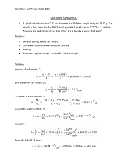


© Copyright 2025